Arc Length and Surface Area

Section 6.5 Arc Length and Surface Area

We’re going to continue to think about different applications of definite integrals: what they can measure and how we can construct these integral formulas. In this section, we’re going to add two more formulas for two more measurements. Before we get far into this discussion, we want to center the important parts of our discussion.

🔗

Sure, it is worth noting that, in this section, we’ll add a 1-dimensional measurement of size to our list of things an integral can measure. We have talked about a 2-dimensional measure of size (area) and a 3-dimensional measure of size (volume), but we’ll add length to the list now! We’ll also add a 2-dimensional extension of perimeter to the list when we talk about surface area. That’s cool!

🔗

But, more importantly, we’re going to see how we can construct an integral formula from a Riemann sum, and we’re going to get some experience constructing a Riemann sum to measure the thing we care about. In our study of integrals, it might not actually be that important to know how to calculate the specific kinds of volumes or lengths that we’re talking about. But we can get some experience with using some formulas from a pretty comfortable field (geometry) to get some experience with the slice-and-sum process. And this process is a useful one to know! We want to see that a definite integral is more than just an area under a curve, and we want to be able to look at an integral formula for some measurement or calculation and see some of the parts of that formula that could be familiar.

🔗

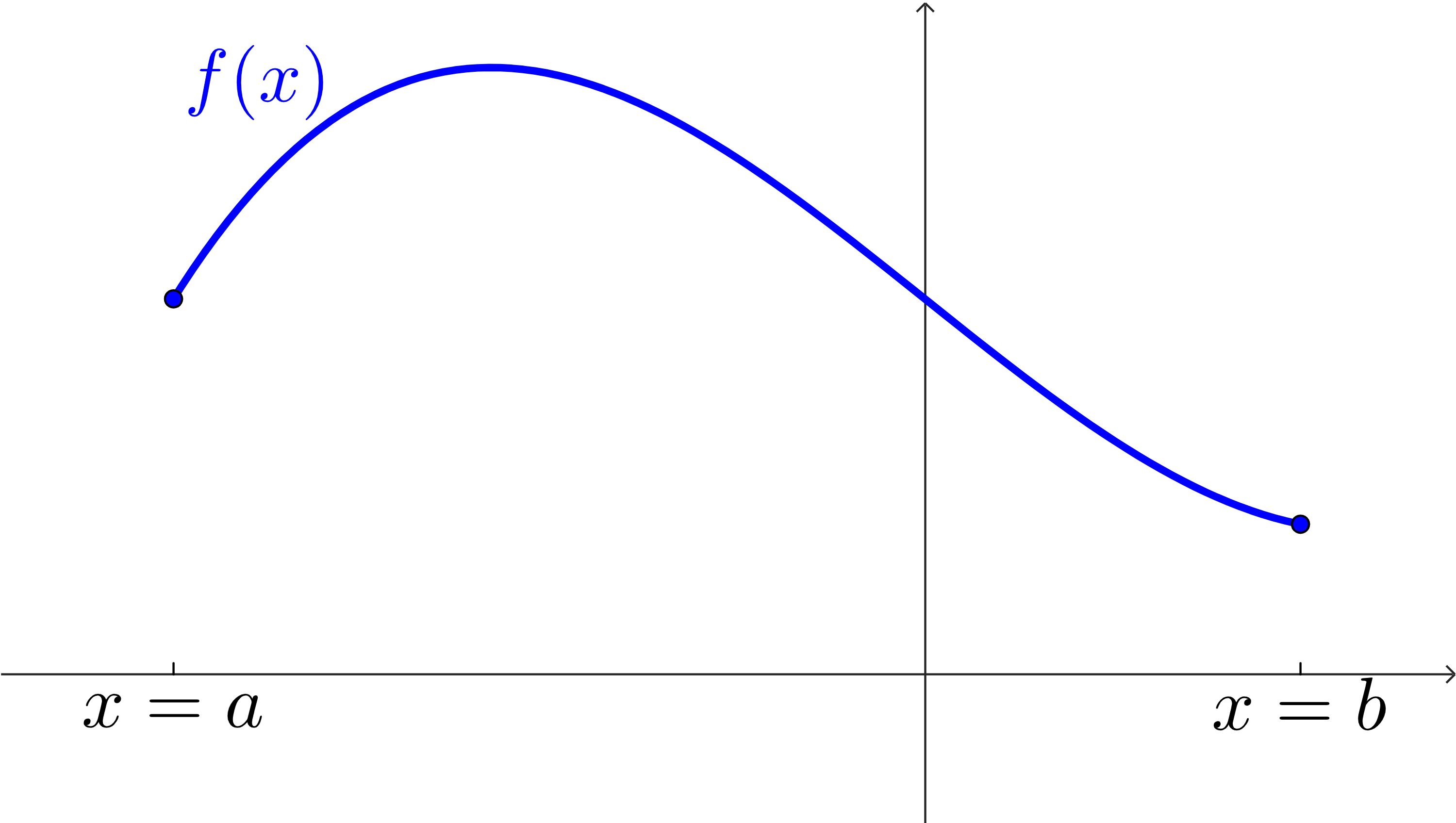
Anyways, let’s calculate some arc lengths.

🔗

Subsection Integrals for Evaluating the Length of a Curve

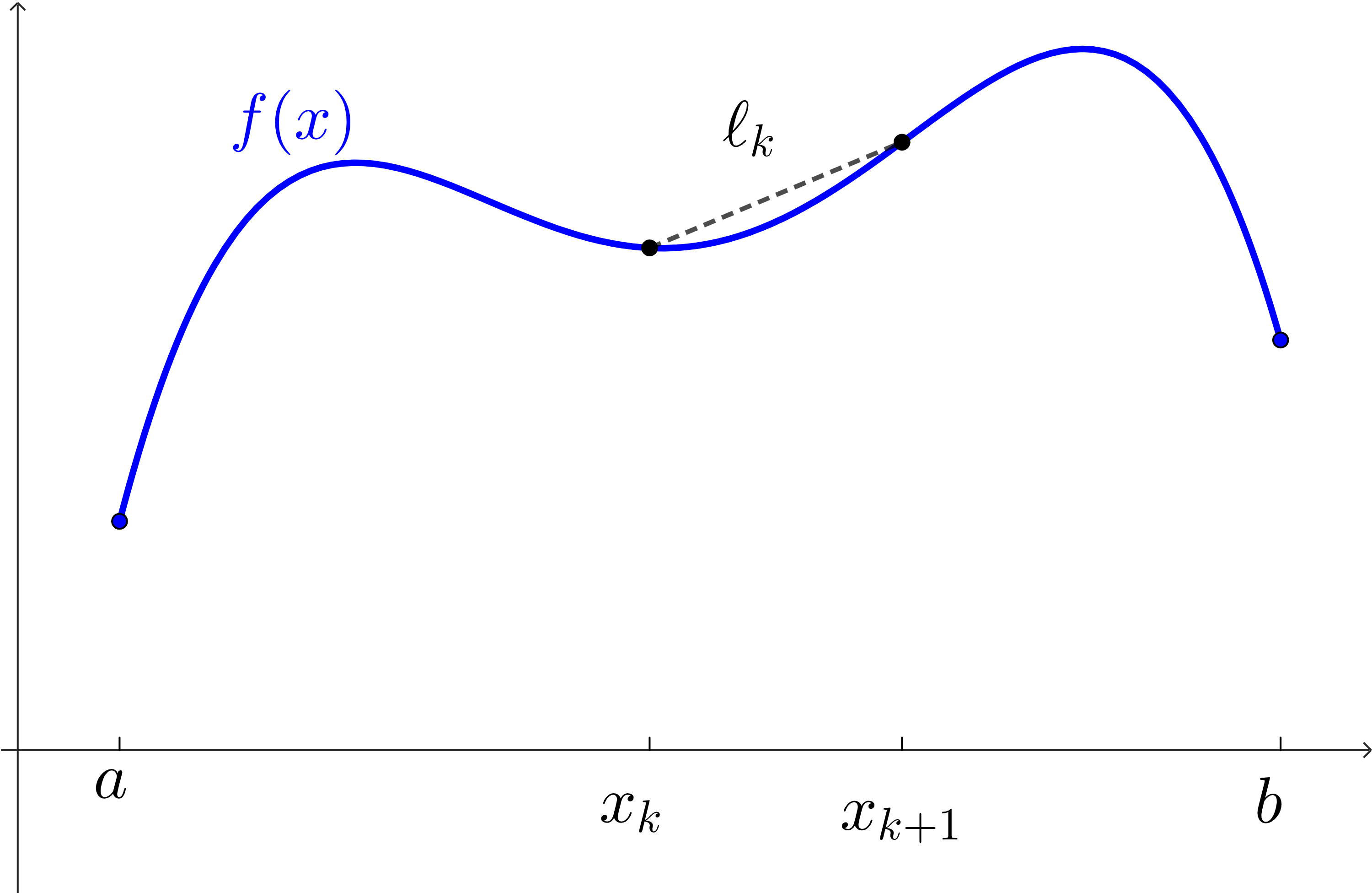
When we talk about arc length, we might think of the length of some portion of a circle. Here, we’ll use it to refer to the length of some more general curve. We’ll graph a function and think about how long the curve of the graph is from some point to another point.

🔗

Activity 6.5.1. Measuring Distance.

(a)

Consider the following right-triangle with the normal names of side lengths.

🔗

A right triangle with the hypotenuse labeled c and the two other side lengths labeled a and b. — Figure 6.5.1.
🔗

How do we use the Pythagorean Theorem to find the length of \(c\text{?}\)

🔗

(b)

Consider the two points \((x_1,y_1)\) and \((x_2, y_2)\) below.

🔗

Two points, (x_1, y_1) and (x_2, y_2), connected by a dashed line. The line is labeled d. — Figure 6.5.2.
🔗

How do we use the distance formula to find the length of the line connecting the two points, \(d\text{?}\)

🔗

(c)

How are these two things the same? How are they different?

🔗

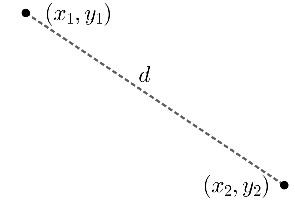
This might be a reminder of something we already knew, but let’s make sure we are certain: when we calculate distances, we’re really just using the Pythagorean Theorem! We can square the vertical distance between the points and the horizontal distance between the points, and then the length of the straight line connecting two points is:

\begin{equation*} \ell = \sqrt{(\Delta x)^2 + (\Delta y)^2}\text{.} \end{equation*}

This will be a useful formula for us to find an integral expression for the length of a curve.

🔗

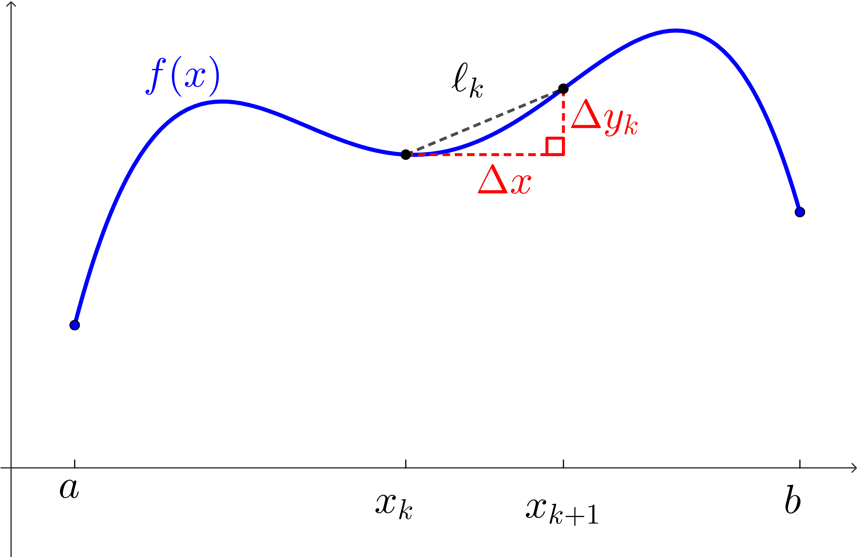
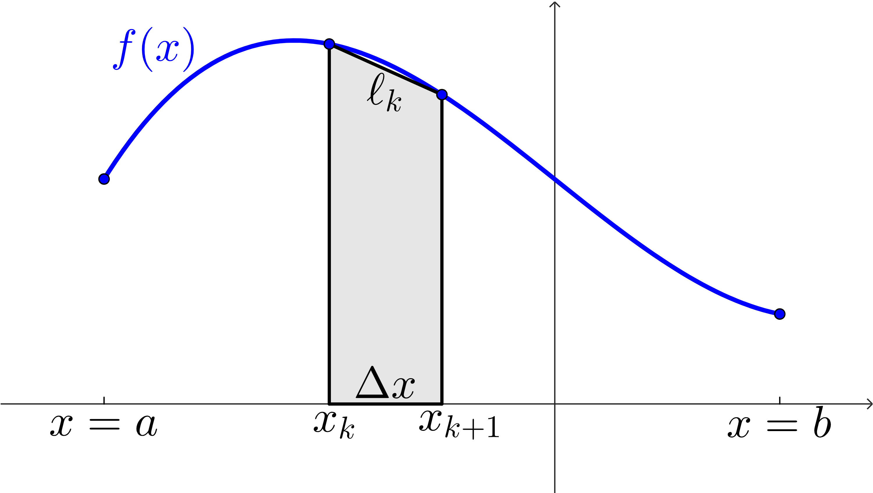
If we think about the slice-and-sum technique, then we’ll want to visualize the \(k\)th slice of whatever we’re trying to measure. In this case, that means we’ll divide the curve up into equally-wide slices and calculate the length of each subsection of the curve. We’ll make a recognizable assumption: we’ll assume that the curve is actually a straight line between the end points, and calculate that length.

🔗

Let’s visualize the \(k\)th slice.

🔗

A curvy, blue function labeled f(x) plotted from a starting point (at x=a) to some ending point (at x=b). Along the way, there are two more points forming an interval from x=x_k to x=x_(k+1). These two points are connected by a straight, dashed line labeled l_k. — Figure 6.5.3.
🔗

In order to calculate \(\ell_k\text{,}\) the straight-line length connecting the end points of the \(k\)th subinterval, we can use the Pythagorean Theorem or distance formula (from Activity 6.5.1).

🔗

Let’s start the slice-and-sum process.

\begin{align*} \ell_k \amp = \sqrt{(\Delta x)^2+(\Delta y_k)^2} \\ \ell \amp \approx \sum_{k=1}^{n}\sqrt{(\Delta x)^2+(\Delta y_k)^2} \end{align*}

Two notes:

We’re using \(\Delta y_k\) to denote the vertical distance between the end points of the \(k\)th subinterval because we expect these to differ for each subinterval. We don’t need to do this for \(\Delta x\text{,}\) since we’ve been slicing things into equally-wide subintervals this whole time.
🔗

🔗
This isn’t a Riemann sum. This is much more important, and much more pressing.
🔗

🔗

Before we can do anything, we need to try to manipulate this sum so that it is in the form of a Riemann sum. What does this mean? What are some of the things required for the Riemann sum structure that we don’t have here? Feel free to look back at Definition 5.2.3 Riemann Sum to remind yourself what elements are needed for a Riemann sum.

🔗

Notice, first, that we need a function evaluated at any single input on the subinterval: \(f(x_k^*)\text{.}\) In our version, we have a function evaluated twice at very specific inputs:

\begin{equation*} \Delta y_k = f(x_{k+1}) - f(x_k)\text{.} \end{equation*}

We’ll need to rethink about how we represent this part in order to get a single function output.

🔗

We also need to have this function multiplied by \(\Delta x\text{.}\) In our sum, we have \(\Delta x\) as a part of the function itself, under the square root. We’ll want to move this \(\Delta x\) outside of the root. Let’s start there.

🔗

We’ll start by looking at the sum to approximate the length \(\ell\) and factoring \(\Delta x\) outside of the root.

\begin{align*} \ell \amp \approx \sum_{k=1}^n \sqrt{(\Delta x)^2+(\Delta y_k)^2}\\ \amp = \sum_{k=1}^{n} \sqrt{(\Delta x)^2\left(1 + \frac{(\Delta y_k)^2}{(\Delta x)^2}\right)}\\ \amp \sum_{k=1}^{n}\Delta x \sqrt{1+\left(\frac{\Delta y_k}{\Delta x}\right)^2}\\ \ell \amp \approx \sum_{k=1}^n \sqrt{1+\left(\frac{\Delta y_k}{\Delta x}\right)^2} \Delta x \end{align*}

This looks better! We have \(\Delta x\) floating around at the end of our sum, ready to turn into \(dx\) once we apply the limit as \(n\to\infty\text{.}\)

🔗

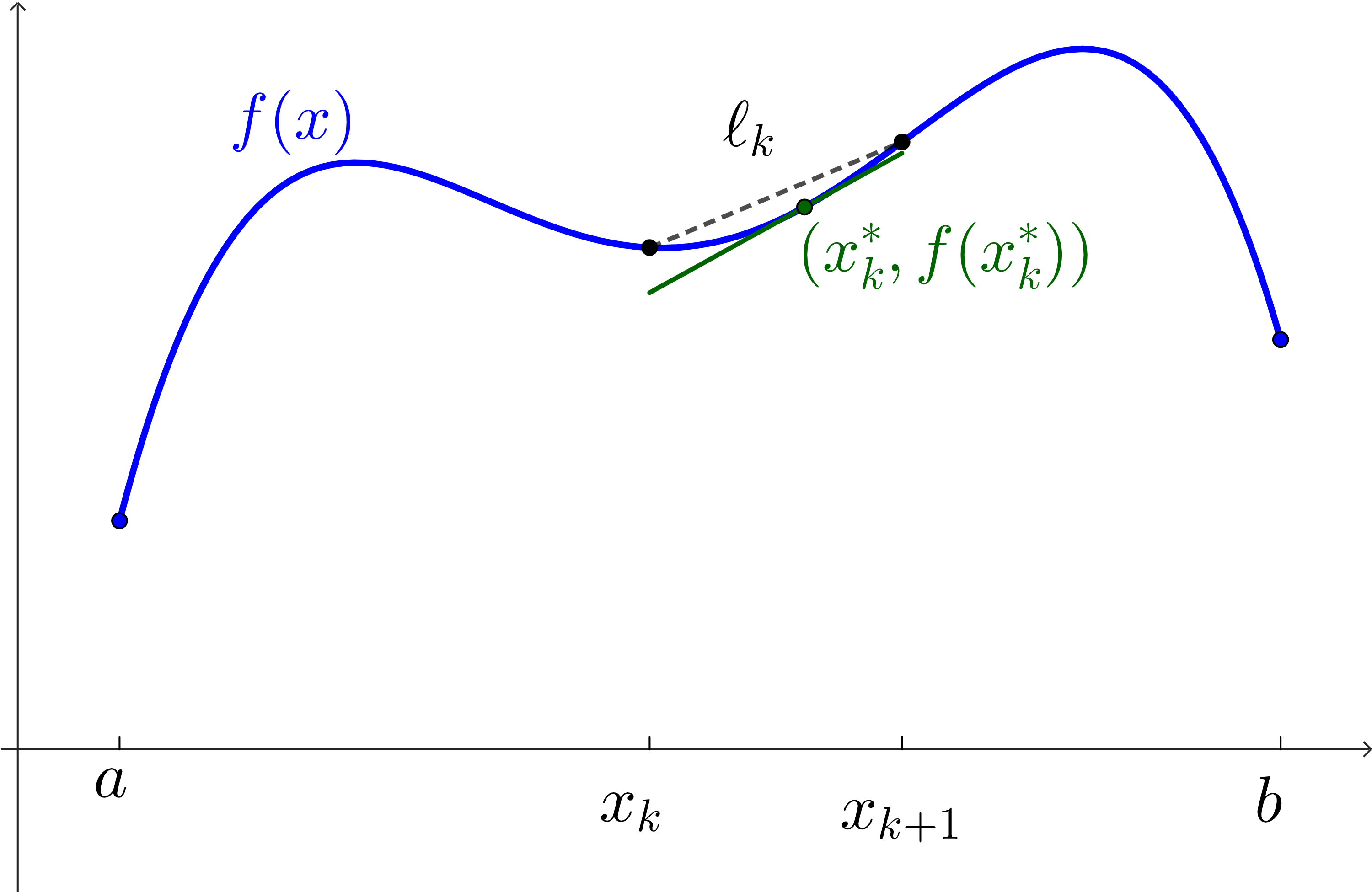
The inside of our root, though, is still a bit messed up. We would like a single function of \(x_k^*\text{,}\) any \(x\)-value from the \(k\)th subinterval. Instead, we have a function involving the two \(x\)-values of the end points and we still have \(\Delta x\) involved in this part!

🔗

But we can notice something about \(\frac{\Delta y_k}{\Delta x}\text{:}\) it really is the slope of the straight line! Can we use a function to represent this? We absolutely can approximate this slope using a function: the derivative!

🔗

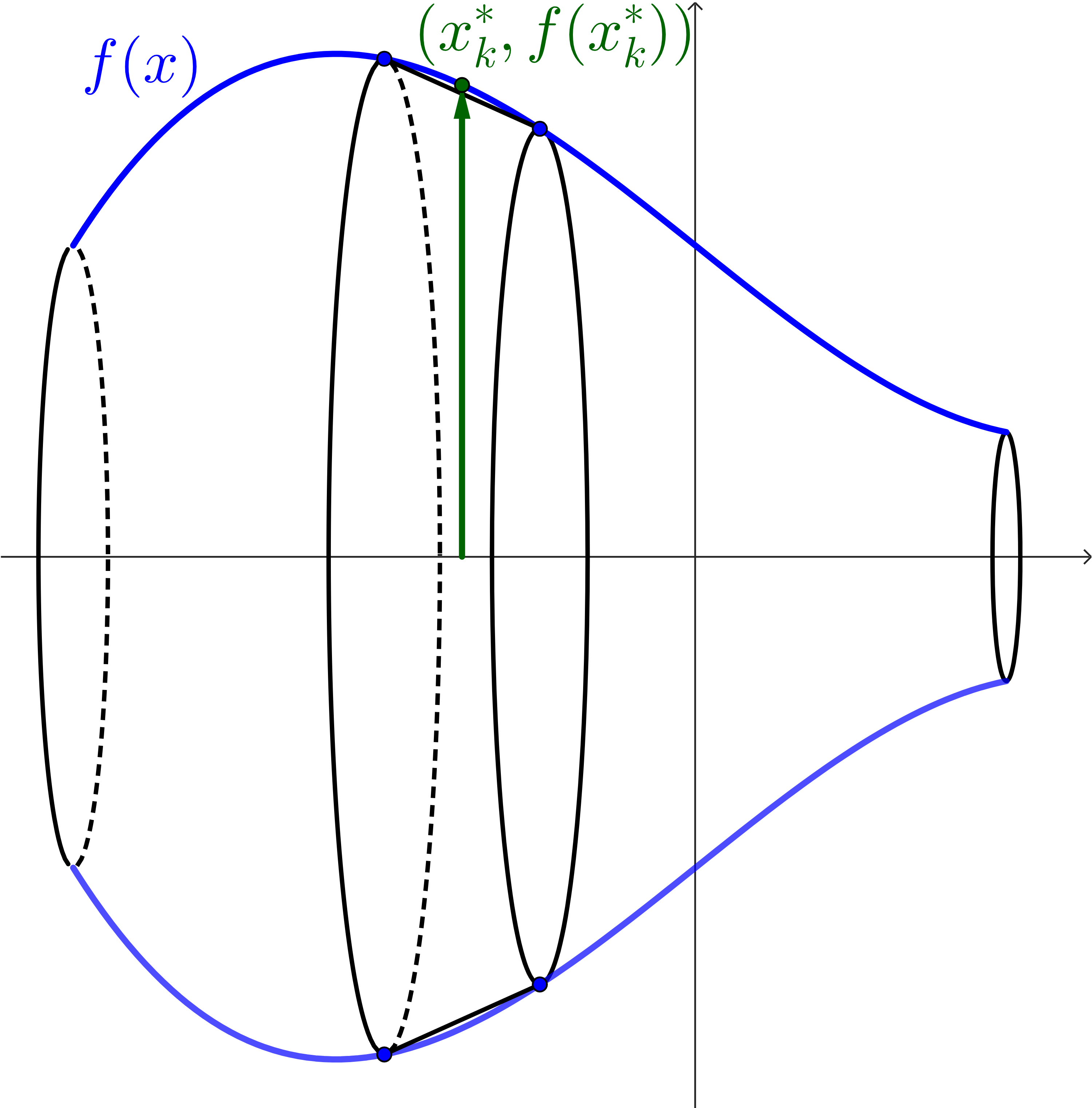
If we pick some point, \((x_k^*, f(x_k^*))\text{,}\) on the \(k\)th subinterval, then we can approximate \(\frac{\Delta y_k}{\Delta x}\) with \(f'(x_k^*)\text{.}\) This is a fine approximation of this slope (and the Mean Value Theorem guarantees that there is a point on the subinterval where \(f'(x_k^*) = \frac{\Delta y_k}{\Delta x}\) exactly), but the real magic will happen when \(n\to\infty\text{.}\) The definition of the Derivative at a Point will make sure that these slopes are equal in the limit!

🔗

Let’s return to our slice-and-sum process.

\begin{align*} \ell \amp \approx \sum_{k=1}^n \sqrt{1+\left(\frac{\Delta y_k}{\Delta x}\right)^2} \Delta x \\ \amp \approx \sum_{k=1}^n \sqrt{1+(f'(x_k^*))^2}\Delta x \end{align*}

This is a Riemann sum! We can apply a limit and get an integral!

\begin{align*} \ell \amp \approx \sum_{k=1}^n \sqrt{1+(f'(x_k^*))^2}\Delta x\\ \ell \amp = \lim_{n\to\infty}\sum_{k=1}^n \sqrt{1+(f'(x_k^*))^2}\Delta x\\ \amp = \int_{x=a}^{x=b} \sqrt{1+(f'(x))^2}\;dx \end{align*}

🔗

Definition 6.5.6. Length of a Curve.

If \(f(x)\) is continuous on the interval \([a,b]\) and differentiable on \((a,b)\text{,}\) then the length of the curve \(y=f(x)\) from \(x=a\) to \(x=b\) is:

\begin{equation*} \int_{x=a}^{x=b}\sqrt{1+(f'(x))^2}\;dx\text{.} \end{equation*}

🔗

Example 6.5.7.

Find an integral expression representing the length of the following curves.

🔗

(a)

The curve \(y=\dfrac{1}{x}\) from \(x=1\) to \(x=2\text{.}\)

🔗

Solution.

Since \(y'=-\dfrac{1}{x^2}\text{,}\) then we can construct the following integral:

\begin{align*} \ell \amp = \int_{x=1}^{x=2}\sqrt{1+(y')^2}\;dx\\ \amp = \int_{x=1}^{x=2} \sqrt{1+\left(-\frac{1}{x^2}\right)^2}\;dx\\ \amp = \int_{x=1}^{x=2}\sqrt{1+\frac{1}{x^4}}\;dx \end{align*}

Instead of worrying about actually evaluating this integral, we’ll leave it like this.

🔗

If you do want to fiddle with this integral, than it might be helpful to note that we can rewrite it:

\begin{align*} \int_{x=1}^{x=2}\sqrt{1+\frac{1}{x^4}}\;dx \amp = \int_{x=1}^{x=2}\sqrt{\frac{x^4+1}{x^4}}\;dx \\ \amp = \int_{x=1}^{x=2} \frac{\sqrt{1+x^4}}{x^2}\;dx \end{align*}

🔗

(b)

The curve \(y=\sin^{-1}(x)\) from \(x=-1\) to \(x=1\text{.}\)

🔗

Solution.

We know that \(y'=\dfrac{1}{\sqrt{1-x^2}}\text{,}\) so we can construct the following integral:

\begin{align*} \ell \amp = \int_{x=-1}^{x=1} \sqrt{1+\left(\frac{1}{\sqrt{1-x^2}}\right)^2}\;dx\\ \amp = \int_{x=-1}^{x=1} \sqrt{1+\frac{1}{1-x^2}}\;dx \end{align*}

We can leave this integral like this for now.

🔗

Similar to the first example, though, we can rewrite this if you’d like to explore it more!

\begin{align*} \int_{x=-1}^{x=1} \sqrt{1+\frac{1}{1-x^2}}\;dx \amp = \int_{x=-1}^{x=1} \sqrt{\frac{2-x^2}{1-x^2}}\;dx \end{align*}

🔗

Subsection Integrals for Evaluating the Surface Area of a Solid

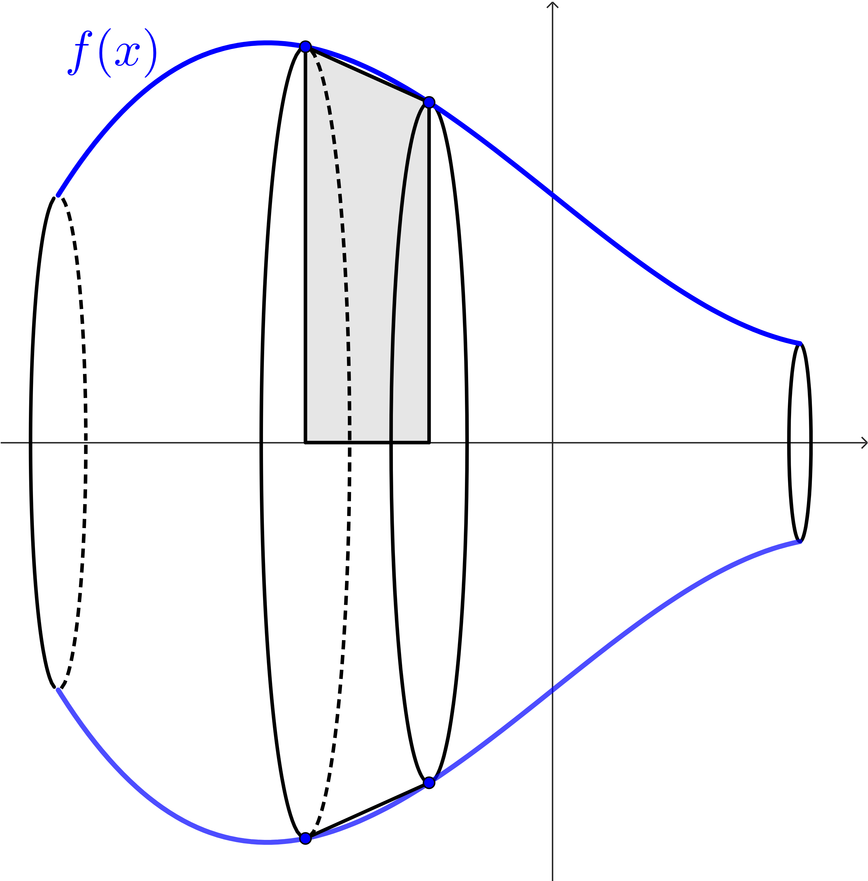
Moving from the length of some curve towards calculating the surface area of some solid of revolution won’t be hard: we’ll use the length formula in our procedure!

🔗

Let’s build this surface area formula. Consider some function, \(f(x)\text{,}\) on the interval from \(x=a\) to \(x=b\text{.}\)

🔗

A blue curve labeled f(x) spanning from a point at x=a to a point at x=b. The curve is above the x-axis. — Figure 6.5.8.
🔗

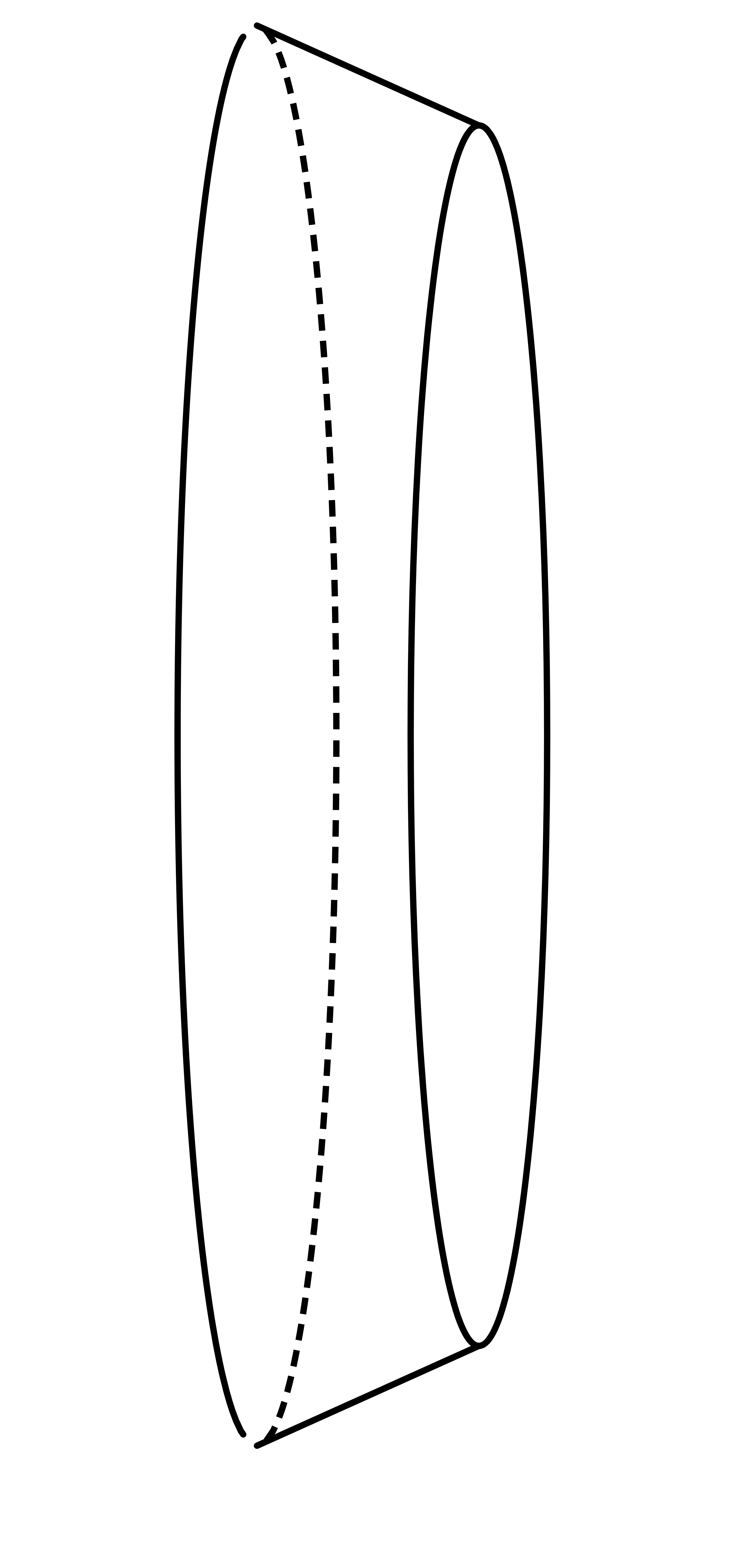
Instead of forming a rectangle for the \(k\)th slice, we’ll do the same thing that we did for arc length: we’ll connect the end points of the \(k\)th subinterval. This will create a trapezoid.

🔗

The same blue curve f(x). There are two more points along the curve connected by a straight line, and a shaded in trapezoid spanning from the diagonal line to the x-axis. The diagonal line of the trapezoid is labeled l_k, while the bottom spans from x_k to x_(k+1) and is labeled Delta x. — Figure 6.5.9.
🔗

We’ll use \(\ell_k\) to represent the diagonal length of the line connecting the endpoints. Notice that this is going to become the arc length.

🔗

When we revolve the curve \(y=f(x)\) around the \(x\)-axis, we can see not just the solid created by the curve, but the solid representing this \(k\)th slice.

🔗

A vase-like shape formed by the blue curve f(x) being revolved around the x-axis. The trapezoid is still pictured, and we can see the circular curves formed when it revolves around the x-axis. It creates a slice that looks like a trapezoidal-cylinder type shape. — Figure 6.5.10.
🔗

The kth slice, looking like a trapezoidal-cylinder type shape, with the radius on one side bigger than the other. — Figure 6.5.11. The \(k\)th frustum-shaped slice.
🔗

In order for us to find the surface area of this \(k\)th slice, we’ll think about how "far" the diagonal line revolves. This is based on the circumference of each circular end of our slice, which means we have two radii to consider: the function outputs at both endpoints of the \(k\)th subinterval:

\begin{equation*} A_k = 2\pi\left(\frac{f(x_k)+f(x_{k+1})}{2}\right)\ell_k \end{equation*}

This is going to become problematic, since we need only one function output evaluated at some \(x_k^*\) on the \(k\)th subinterval.

🔗

Instead, we can select some \(x\)-value on the interval and use the function output at that point to represent the radius of our \(k\)th slice.

🔗

The solid formed by f(x) being revolved around, and the kth slice visualized. There is also a green arrow pointing from the x-axis to a point on the kth interval labeled (x_k^*, f(x_k^*)) acting as a radius of the sliced solid. — Figure 6.5.12.
🔗

Instead of averaging the large and small radii from the end-points, we’ll just select the one function output to represent this "average" radius. In the limit as \(n\to\infty\text{,}\) things will work out, since this randomly selected radius will become exactly equal to the average radius in the limit since \(\Delta x\to 0\text{.}\)

🔗

Now we can slice and sum!

\begin{align*} A_k \amp = 2\pi f(x_k^*)\ell_k \\ \amp = 2\pi f(x_k^*) \sqrt{1+(f'(x_k^*))^2}\Delta x\\ A \amp \approx \sum_{k=1}^n 2\pi f(x_k^*) \sqrt{1+(f'(x_k^*))^2}\Delta x\\ A \amp = \lim_{n\to\infty} \sum_{k=1}^n 2\pi f(x_k^*) \sqrt{1+(f'(x_k^*))^2}\Delta x\\ \amp = \int_{x=a}^{x=b} 2\pi f(x)\sqrt{1+(f'(x))^2}\;dx \end{align*}

🔗

Definition 6.5.13. Surface Area.

Let \(f(x)\) be a continuous function with \(f(x)\geq 0\) on the interval \([a,b]\) and differentiable on \((a,b)\text{.}\) If the region bounded by \(f(x)\) and the \(x\)-axis from \(x=a\) to \(x=b\) is revolved around the \(x\)-axis, then the surface area of the resulting solid is:

\begin{equation*} A = 2\pi\int_{x=a}^{x=b} f(x)\sqrt{1+(f'(x))^2}\;dx\text{.} \end{equation*}

🔗

Practice Problems Practice Problems

1.

The formula for arc length of the function \(f(x)\) on the interval \([a,b]\) is \(\displaystyle L = \int_{x=a}^{x=b} \sqrt{1+f'(x)^2}\;dx\text{.}\) Explain how this definition is built, using the slice-and-sum method. Make sure to explain how we the Pythagorean Theorem is involved.

🔗

2.

Why do we use \(f'(x)\) in the formula for arc length?

🔗

3.

For each of the following curves on intervals, evaluate the arc length.

🔗

(a)

\(y = -6x+2 \) on \([1,5]\)

🔗

(b)

\(y=\dfrac{x^{3/2}}{3}\) on \([0,60]\)

🔗

(c)

\(y=\dfrac{x^4}{4}+ \dfrac{1}{8x^2}\) on \([1,3]\)

🔗

4.

For each of the following curves on intervals, set up an integral representing the arc length. Do not evaluate.

🔗

(a)

\(y=\tan^2(x)\) on \(\left[-\frac{\pi}{4}, \frac{\pi}{4}\right]\)

🔗

(b)

\(y=\ln(x^2)\) on \([1, e]\)

🔗

(c)

\(y = \sqrt{x+1}\) on \([-1,8]\)

🔗

5.

Why is the formula for arc length seemingly involved in the integral formula for surface area of a solid of revolution?

🔗

6.

In the integral formula \(\displaystyle A = \int_{x=a}^{x=b} 2\pi f(x) \sqrt{1+f'(x)^2} \; dx\text{,}\) what does \(f(x)\) represent? What about \(2\pi\text{?}\)

🔗

7.

For each of the following curves and intervals, find the surface area of the solid formed when the curve is revolved around the \(x\)-axis.

🔗

(a)

\(y = 2x+3\) on \([0,3]\)

🔗

(b)

\(y = 4\sqrt{x}\) on \([4, 9]\)

🔗

(c)

\(y=\dfrac{x^4}{4}+ \dfrac{1}{8x^2}\) on \([1,3]\)

🔗

8.

For each of the following curves and intervals, set up the surface area of the solid formed when the curve is revolved around the \(x\)-axis. Do not evaluate the integral.

🔗

(a)

\(y = \sin\left(e^{x^2}\right)+1\) on \([0,2]\)

🔗

(b)

\(y = \ln(x^2)\) on \([1,e]\)

🔗

Prev Top Next