Continuity and the Intermediate Value Theorem

Section 1.6 Continuity and the Intermediate Value Theorem

What does it mean for a function to be continuous?

This might be a familiar concept to you, and we all probably have some idea of what the word “continuous” means (or should mean), both in a colloquial context and in a math-specific context. Instead of focusing on some of the traditional ideas like “can you draw the graph without picking up your pencil”, we’re going to formalize the idea of continuity a bit.

🔗

And the first thing that we’ll have to do is shift our intuition from what continuity is describing. We won’t (at least at first) use continuity as a classification of functions, as a whole. Instead, we’re going to think of continuity as a description of some “local” behavior.

🔗

Subsection Continuity as Connectedness

We’re going to try to think about what we want to describe when we define continuity. The description of “drawing a graph without picking up a pencil” is a global property, and also a pretty vague and ambiguous one.

🔗

Activity 1.6.1. Classification and Continuity.

Let’s consider the following functions, graphed below.

🔗

A graph of a function with a vertical asymptote and a horizontal asymptote. — Figure 1.6.1. A variety of graphs for us to use to think about continuity.
🔗

A graph of a function that increases from (0,0) onward. — Figure 1.6.1. A variety of graphs for us to use to think about continuity.
🔗

(a)

Can you point out any points on the functions above that seem like the functions might not be continuous? Note that we’re not classifying each function as “continuous” or “not continuous”!

🔗

(b)

We want to build towards a definition of continuity using “connectedness” as the key: a function is continuous at a point if it is connected to itself. How does that work when we think about function values and limits? Use the graphs above and the points you looked at to help!

🔗

There are definitely some unknowns here. One of the questions that students ask a lot during an investigation like this is what we do about end-points. Is a function continuous at a closed ending-point in its domain? Is it connected to itself? To answer questions like this, we should try to write out what we mean by connectedness.

🔗

A pretty basic version of this is something like “A function is connected to itself at a point if, for the inputs near that point, the function values are close to the function value at the point.” Maybe even more concise is “Small deviations in the inputs produce small changes in the outputs.”

🔗

Subsection Defining Continuity

We’re going to take this idea of a function being connected to itself as “small deviations in the inputs produce small changes in the outputs” and write it down using limit notation.

🔗

Definition 1.6.2. Continuous at a Point.

The function \(f(x)\) is continuous at an \(x\)-value in the domain of \(f(x)\) if \(x=a\) if \(\displaystyle \lim_{x\to a}f(x)=f(a)\text{.}\)

🔗

If \(f(x)\) is not continuous at \(x=a\text{,}\) but one of the one-sided limits is equal to the function output, then we can define directional continuity at that point:

We say \(f(x)\) is continuous on the left at \(x=a\) when \(\displaystyle \lim_{x\to a^-} f(x)=f(a)\text{.}\)
🔗

🔗
We say \(f(x)\) is continuous on the right at \(x=a\) when \(\displaystyle \lim_{x\to a^+} f(x)=f(a)\text{.}\)
🔗

🔗

🔗

In using limits, we get some flexibility: we can talk about one-sided limits, specifically! This helps us take care of the pesky “Is a function connected to itself at a closed ending point,” question! We can say, using this definition, “Yes, on the left side!” or “Yes, on the right side!”

🔗

Example 1.6.3.

For the function \(f(x)\) defined below, decide whether or not the function is continuous at the point listed. If it is not continuous, report whether it is continuous on one side.

\begin{equation*} f(x) = \begin{cases} 2x+1 \amp \text{when } x\leq 2\\ \dfrac{2x^2+7}{3} \amp \text{when } 2\lt x \lt 4\\ \dfrac{6}{x-1} + 3 \amp \text{when } x\geq 4 \end{cases} \end{equation*}

🔗

(a)

Is \(f(x)\) continuous at the point \((2,5)\text{?}\)

🔗

Hint.

Check the one-sided limits as \(x\to 2\text{.}\) Do they both equal \(5\text{?}\) Does one of them?

🔗

Solution.

\begin{align*} \lim_{x\to 2^-} f(x) \amp = \lim_{x\to 2^-} 2x+1\\ \amp = 2(2)+1\\ \amp = 5\\ \lim_{x\to 2^+} f(x)\amp \lim_{x\to 2^+} \frac{2x^2+7}{3} \\ \amp = \frac{2(2)^2+7}{3}\\ \amp = 5 \end{align*}

So \(\displaystyle\lim_{x\to 2}f(x) = 5\text{.}\) Since \(f(2)=5\) as well, we have \(\displaystyle\lim_{x\to 2}f(x) = f(2)\) which means that \(f(x)\) is continuous at \(x=2\text{.}\)

🔗

(b)

Is \(f(x)\) continuous at the point \((4, 5)\text{?}\)

🔗

Hint.

Check the one-sided limits as \(x\to 4\text{.}\) Do they both equal \(5\text{?}\) Does one of them?

🔗

Solution.

\begin{align*} \lim_{x\to 4^-} f(x) \amp = \lim_{x\to 4^-} \frac{2x^2+7}{3}\\ \amp = \frac{2(4)^2+7}{3}\\ \amp = 13\\ \lim_{x\to 4^+} f(x) \amp = \lim_{x\to 4^+} \frac{6}{x-1} + 3\\ \amp = \frac{6}{4-1}+3\\ \amp = 5 \end{align*}

Since \(\displaystyle \lim_{x\to 4^-} f(x) \neq \lim_{x\to 4^+} f(x) \) we know that \(\displaystyle\lim_{x\to 4} f(x) \) doesn’t exist, and so this function cannot be continuous at \(x=4\text{.}\)

🔗

But we can notice that \(\displaystyle\lim_{x\to 4^+} f(x) =f(4)\text{,}\) and so we can say that the function is still continuous on the right side at \(x=4\text{.}\)

🔗

Another bit of flexibility that we have with this definition is that, once we know whether a function is continuous at a point or not, we can string together points in an interval and classify a function as continuous on an interval.

🔗

Definition 1.6.4. Continuous on an Interval.

We say that \(f(x)\) is continuous on the interval \((a,b)\) if \(f(x)\) is continuous at every \(x\)-value with \(a\lt x \lt b\text{.}\)

🔗

If \(f(x)\) is continuous on the right at \(x=a\) and/or continuous on the left at \(x=b\text{,}\) then we will say that \(f(x)\) is continuous on the interval \([a,b)\text{,}\) \((a,b]\text{,}\) or \([a,b]\text{,}\) whichever is relevant.

🔗

Something to notice, here, is that we won’t do this by checking each individual \(x\)-value in an interval. If we wanted to say that a function was continuous on \((0,1)\text{,}\) we would then have to consider every real number between \(0\) and \(1\text{.}\) But there are an infinite amount of these!

🔗

So when we talk about a function being continuous on an interval, we’ll really think about this by pointing out the places where a function is not continuous (\(x\)-values where \(f(x)\) violates some part of Definition 1.6.2).

🔗

Subsection Discontinuities

Since we’ll want to label functions at places that they are not continuous (in order to write the intervals where it is continuous), we should summarize some things about discontinuities.

🔗

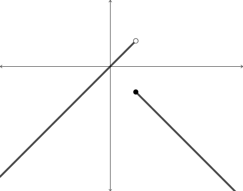
Where is a Function not Continuous?

Most of the functions that we consider in this text will be continuous everywhere that it makes sense: on their domain. That is, if there is a point defined at some \(x\)-value, it is likely that the function’s limit matches the \(y\)-value of the point. More specifically, though:

A function is discontinuous at any location that results in an infinite limit. These are locations where \(f(x)\) is undefined and the limit is infinite (and so doesn’t exist).
🔗

🔗
A function is, in general, discontinuous at any \(x\)-value where \(f(x)\) is not defined. This seems silly to say! We probably could have left this unsaid. Of course \(f\) isn’t continuous at an \(x\)-value not in its domain.
🔗

🔗
A function that is defined as a piecewise function could be discontinuous at locations where the pieces meet: maybe the limit doesn’t exist, or maybe the function value is not defined, or maybe the limit exists and the function value is defined but they do not match.
🔗

🔗

🔗

Some quick notes:

Every polynomial function is continuous everywhere on its domain. We knew this already, from Theorem 1.2.7 Limits of Polynomials: the limit is always the same as the function value at any input!
🔗

🔗
Rational functions are only discontinuous when there is division by 0.
🔗

🔗
Even-root functions (like square roots) are continuous whenever the radicand (the stuff under the root) is positive. We might need to investigate wherever the radicand is equal to \(0\text{,}\) since the function might only be continuous on one side.
🔗

🔗
The following functions are continuous on their domains:
- \(y=\sin(x)\) on \((-\infty,\infty)\)
  🔗
  
  🔗
- \(y=\cos(x)\) on \((-\infty,\infty)\)
  🔗
  
  🔗
- \(y=e^x\) on \((-\infty,\infty)\)
  🔗
  
  🔗
- \(y=\ln(x)\) on \((0,\infty)\)
  🔗
  
  🔗
🔗
🔗

🔗

Example 1.6.5.

Let’s revisit the same function we looked at earlier:

\begin{equation*} f(x) = \begin{cases} 2x+1 \amp \text{when } x\leq 2\\ \dfrac{2x^2+7}{3} \amp \text{when } 2\lt x \lt 4\\ \dfrac{6}{x-1} + 3 \amp \text{when } x\geq 4 \end{cases} \end{equation*}

🔗

We already looked at what was happening at \(x=2\) and \(x=4\text{.}\) Are there any other \(x\)-values where this function might not be continuous? Why or why not? Can you report the intervals on which \(f(x)\) is continuous?

🔗

Hint.

Can you name the function type for \(x\lt 2\text{,}\) \(2\lt x\lt 4\) and \(x\gt 4\text{?}\)

🔗

Solution.

Since \(f(x)\) is polynomial for \(x\lt 2\) and \(2\lt x\lt 4\text{,}\) we know that the function is continuous on those intervals as well. We can see that for \(x\gt 4\text{,}\) \(f(x)\) is a rational function. Since the only \(x\)-value where we might divide by 0 is outside of the interval for which this function part is defined, we know that this function is continuous for \(x\gt 4\text{.}\)

🔗

Since our function is continuous at \(x=2\text{,}\) we can say that it is continuous on the interval \((-\infty, 4)\text{.}\) We also say that the function was continuous on the right at \(x=4\text{,}\) and so we can say that \(f(x)\) is also continuous on the interval \([4,\infty)\text{.}\)

🔗

We’ll end this section with one last result that will be pretty important. Continuity, as a property, will be useful as we move forward, but only for a few specific reasons. One is the following result.

🔗

Theorem 1.6.6. Continuity with Composition.

For two functions \(f(x)\) and \(g(x)\text{,}\) if \(\displaystyle\lim_{x\to a}g(x)=L\) and \(f(x)\) is continuous at \(x=L\text{,}\) then

\begin{equation*} \lim_{x\to a} f(g(x)) = f\left(\lim_{x\to a}g(x)\right) = f(L)\text{.} \end{equation*}

🔗

This is a generalization of the properties of limits that we explored earlier (Theorem 1.2.5 Combinations of Limits). We can use this new theorem to evaluate limits by just noticing if pieces of our function might behave nicely with limits.

🔗

Let’s evaluate the following limit:

\begin{equation*} \lim_{x\to 1}\left(\sin\left(\sqrt{e^{x^2-2x+1}}\right)\right)\text{.} \end{equation*}

Notice that the sine function is continuous everywhere. This means that we can bring the limit statement “inside” by a layer:

\begin{equation*} \lim_{x\to 1}\left(\sin\left(\sqrt{e^{x^2-2x+1}}\right)\right) = \sin\left(\lim_{x\to 1}\sqrt{e^{x^2-2x+1}}\right)\text{.} \end{equation*}

Now we can think about the square root function: we know that the radicand function (the exponential) always produces positive outputs. So we can bring the limit statement “inside” by another layer of composition:

\begin{equation*} \sin\left(\lim_{x\to 1}\sqrt{e^{x^2-2x+1}}\right) = \sin\left(\sqrt{\lim_{x\to 1}e^{x^2-2x+1}}\right)\text{.} \end{equation*}

The exponential function is also continuous everywhere:

\begin{equation*} \sin\left(\sqrt{\lim_{x\to 1}e^{x^2-2x+1}}\right) = \sin\left(\sqrt{e^{\lim_{x\to 1}x^2-2x+1}}\right)\text{.} \end{equation*}

And we also know that polynomial functions are continuous everywhere!

\begin{align*} \sin\left(\sqrt{e^{\lim_{x\to 1}x^2-2x+1}}\right) \amp = \sin\left(\sqrt{e^{(1)^2-2(2)+1}}\right) \\ \amp = \sin\left(\sqrt{e^0}\right)\\ \amp = \sin(1) \end{align*}

This seemingly difficult limit is actually as easy as just evaluating the function at the input, since the function behaves nicely.

🔗

Subsection Intermediate Value Theorem

Let’s introduce one of the biggest results coming from continuity of functions that exists. We’re going to simply state the result and then discuss it, instead of building up towards it.

🔗

Theorem 1.6.7. Intermediate Value Theorem.

If \(f(x)\) is a function that is continuous on \([a,b]\) with \(f(a)\neq f(b)\) and \(L\) is any real number between \(f(a)\) and \(f(b)\) (either \(f(a)\lt L \lt f(b)\) or \(f(b) \lt L \lt f(a)\)), then there exists some \(c\) between \(a\) and \(b\) (\(a\lt c \lt b\)) such that \(f(c)=L\text{.}\)

🔗

This theorem was stated as early as the 5th century BCE by Bryson of Heraclea. Back then, a really interesting problem was related to “squaring the circle.” That is, given a circle with some measurable radius, can we construct a square with equal area? This is obviously true, in that we can just use a square with the side length \(r\sqrt{\pi}\text{.}\) What we typically mean by “construct,” though, is to create this square using only a compass and straightedge (a ruler without length markings) and only a finite number of steps. This was finally proven to be impossible in 1882, approximately 2300 years later.

🔗

Bryson of Heraclea knew that the square itself existed (even if he couldn’t construct it) because he was able to find a circle with area less than the square (by inscribing a circle inside of the square) and a circle with area greater than the square (where the square is inscribed in the circle). Since he posited that he could increase the size of the circle in a continuous manner (without using those words), he claimed that a square with area equal to that of the circle must exist, since the area of the circle passes through all values from the smaller area to the larger area.

🔗

This is a seemingly simple result (even if it is stated in a seemingly complicated way): of course, in order to go from a point at one \(y\)-value to another point at a different \(y\)-value, the function has to pass through all of the \(y\)-values in between. This is pretty obvious, once we see through the phrasing.

🔗

We can use this result in some pretty interesting ways, though! Here’s a favorite:

🔗

Let’s consider two people, standing on polar opposite points on the earth. Let’s say that these two people are carrying thermometers and are measuring the ambient temperature at their location. They coordinate their movement, and begin to move around the earth in a circle, remaining at polar opposite locations as they move.

🔗

How likely is it that the pair finds some location on their path where their temperature readings are exactly identical?

🔗

Let’s pretend that the locations that they start in are different temperatures (or else yay, we found the spot where the temperatures are the same!), and that the starting position of person A is hotter than the starting position of person B.

🔗

Can you see why we are guaranteed that there must be some pair of polar opposite locations where the ambient temperatures are identical?

🔗

If the ambient temperature differs continuously, then the Intermediate Value Theorem says that between the locations where the temperature differential is negative and where it is positive, the temperature differential function must pass through zero!

🔗

This argument can be used in a variety of contexts, and can be used to show that you can typically fix a wobbly table (where the legs don’t all rest nicely on the ground) or chair by rotating it until all of the legs rest nicely on the ground.

🔗

The theorem itself might not seem that interesting, but it’s important both historically and also as a means of making arguments function values, especially when we claim that a function has to be 0 (because we show that there is a point where the function is positive, a point where it is negative, and the function is continuous in between the points).

🔗

Practice Problems Practice Problems

1.

Explain how the definition of continuity (Definition 1.6.2) describes a function being “connected to itself” at the point.

🔗

2.

What does it mean for a function to be continuous on the left at a point? What about on the right?

🔗

3.

Use the definition of continuity at a point to determine whether each function is continuous at the point listed. If it is not, is the function continuous on one side at the point? Explain.

🔗

(a)

\(f(x) = \begin{cases} 4x+1 \amp \text{if } x\lt 1\\ x^2+5 \amp \text{if } x\geq 1 \end{cases}\) at \(x=1\)

🔗

(b)

\(g(x) = \begin{cases} 6x^2-2 \amp \text{if } x\lt0\\ 4 \amp \text{if } x=0\\ 1-3\cos(x) \amp \text{if } x\gt 0 \end{cases}\) at \(x=0\)

🔗

(c)

\(h(x) = \begin{cases} \left(\dfrac{x^2-1}{x+1}\right) \amp \text{if } x\neq -1\\ -2 \amp\text{if } x=-1 \end{cases}\) at \(x=-1\)

🔗

4.

Find the values of \(a\) that make the function continuous at the point that is listed. If no such value of \(a\) exists, say so and explain why.

🔗

(a)

\(f(x) = \begin{cases} x -6\amp \text{if } x\lt3\\ ax^2+1 \amp \text{if } x\geq 3 \end{cases}\) at \(x=3\)

🔗

(b)

\(f(x) = \begin{cases} \dfrac{x^2-4}{x+2} \amp \text{if } x\neq -2\\ a \amp \text{if } x=-2 \end{cases}\) at \(x=-2\)

🔗

5.

Use the properties of composition and continuity to evaluate the following limits.

🔗

(a)

\(\displaystyle \lim_{x\to 0} \left(\sin\left(e^{\sqrt{x^2}}\right)\right)\)

🔗

(b)

\(\displaystyle \lim_{x\to 0} \ln\left(\dfrac{\cos(x^2)}{x^2+1}\right)\)

🔗

(c)

\(\displaystyle \lim_{x\to 0} \sqrt[3]{\dfrac{x}{\sqrt{16x+1}-1}}\)

🔗

6.

“Even a broken clock is right twice a day,” is a common phrase used to say that even an unreliable person can have a good point on accident. Explain how we can use the Intermediate Value Theorem to prove that a broken (analog) clock is guaranteed right twice per day. (Here, we’re assuming that “broken” means stuck.)

🔗

7.

Explain why this argument doesn’t work to show that an unreliable person will be guaranteed to have a good point on accident.

🔗

8.

Prove that at some point in your life you were exactly \(\pi\) feet tall.

🔗

Prev Top Next