Implicit Differentiation

Section 3.1 Implicit Differentiation

Let’s quickly recap what we’ve done with this new calculus object, the derivative:

We defined the derivative at a point (Definition 2.1.1) to find the slope of a line touching a graph of a function \(f(x)\) at a single point. We call this the “slope of the tangent line” at a point.
🔗

🔗
Once we calculated this slope, we quickly found a way to think about the derivative as a function (Definition 2.1.2) that connects \(x\)-values with the slope of the line tangent to \(f(x)\) at that \(x\)-value.
🔗

🔗
We thought about how we could interpret the derivative as more than just a slope (Section 2.2). We can think about this as an instantaneous rate of change, and use it to add detail to how we think about mathematical models of different things.
🔗

🔗
We spent some time building up shortcuts, noticing patterns, and generalizing ways of finding these derivative functions for specific functions (Section 2.3) as well as combinations of those functions (Section 2.4 and Section 2.5).
🔗

🔗

Our goal, now, is to generalize this a bit. What happens when we push past the restriction of only dealing with functions? Can we think of some reasonable non-functions that might produce curves? Might we think about tangent lines and slopes in these contexts?

🔗

Subsection Explicit vs. Implicit Definitions

Definition 3.1.1. Explicitly and Implicitly Defined Curves.

A function or curve that is defined explicitly is one where the relationship between the variables is stated in with an equation like \(y=f(x)\text{.}\) Here, \(x\) is the input variable and we can find each corresponding value of the \(y\)-variable by applying some operations to \(x\text{.}\) As an example, we might consider the following function:

\begin{equation*} y=3x+1\text{.} \end{equation*}

🔗

A function or curve that is defined implicitly is one where the relationship between the variables is stated with an equation connecting the variables, but not necessarily one which is solved for a single variable. Here, the relationship between variables is not stated with the typical input and output variables. As an example, we might consider the same function as above, but defined as:

\begin{equation*} y-3x-1=0\text{.} \end{equation*}

🔗

Often, an implicitly defined curve is one where we cannot solve for a single variable by isolating it.

🔗

A classic and important implicitly defined curve is the unit circle:

\begin{equation*} x^2+y^2=1\text{.} \end{equation*}

We can try to isolate for \(y\) and write this as an explicitly defined curve, and end up with:

\begin{equation*} y=\sqrt{1-x^2}\text{.} \end{equation*}

Unfortunately, this only displays the upper half of the circle, since the square root will only output positive values. In this case, we can get around this by defining the circle with two functions.

🔗

As we move forward, let’s work with this circle using the implicitly defined version (\(x^2+y^2=1\)). How might we find a slope of a line tangent to this circle at some point?

🔗

Subsection Using a Derivative as an Operator

Let’s recall back to Notation for Derivatives. We talked about how we can use the notation \(\ddx{f(x)}\) as a kind of action: the notation says “find the derivative of \(f(x)\) with respect to \(x\text{.}\)” When we say “with respect to \(x\text{,}\)” we mean that we are treating \(x\) as an input variable, and trying to find out how \(f\) changes based on changes to that input. The notation says, “find the rate at which \(f(x)\) changes as \(x\) increases.”

🔗

Because this notation is a call to action, we can use it when we’re dealing with an equation. We can call back to our early algebra days, where we learned that whatever we do to one side of an equation needs to be done to the other side, in order to maintain the equality.

🔗

We can apply this to our derivative actions: we can differentiate both sides of an equation!

🔗

Activity 3.1.1. Thinking about the Chain Rule.

(a)

Explain to someone how (and why) we use the The Chain Rule to find the following derivative:

\begin{equation*} \ddx{\sqrt{\sin(x)}}\text{.} \end{equation*}

🔗

(b)

Let’s say that \(f(x)=\sin(x)\text{.}\) Explain how we find the following derivative:

\begin{equation*} \ddx{\sqrt{f(x)}}\text{.} \end{equation*}

How is this different, or not different, than the previous derivative?

🔗

(c)

Let’s say that we have some other function, \(g(x)\text{.}\) Explain how we find the following derivative:

\begin{equation*} \ddx{\sqrt{g(x)}}\text{.} \end{equation*}

How is this different, or not different, than the previous derivatives?

🔗

(d)

What is the difference between the following derivatives:

\begin{equation*} \ddx{\sqrt{x}} \hspace{0.7cm} \ddx{\sqrt{y}} \hspace{0.7cm} \dd{}{y}\left(\sqrt{y}\right) \end{equation*}

🔗

Hint.

When do we need to use the Chain Rule? When do we need to use some linking derivative to connect the function we’re looking at with the variable we care about?

🔗

Solution.

\begin{align*} \ddx{\sqrt{x}} \amp = \ddx{x^{1/2}}\\ \amp = \frac{1}{2}(x^{-1/2})\\ \amp = \frac{1}{2\sqrt{x}} \end{align*}

🔗

\begin{align*} \ddx{\sqrt{y}} \amp = \dd{}{y}\left(y^{1/2}\right) \cdot \dydx\\ \amp = \frac{1}{2}(y^{-1/2}) \cdot \dydx\\ \amp = \frac{1}{2\sqrt{y}}\cdot \dydx\\ \text{or } \amp \frac{y'}{2\sqrt{y}} \end{align*}

🔗

\begin{align*} \dd{}{y}\left(\sqrt{y}\right) \amp = \ddx{x^{1/2}}\\ \amp = \frac{1}{2}(y^{-1/2})\\ \amp = \frac{1}{2\sqrt{y}} \end{align*}

🔗

Because we’ll be applying our derivative notation to pieces of some equation, we need to be very aware of where we need to apply the Chain Rule.

🔗

Now we can look at some examples of implicitly defined curves and think about questions about the derivative. Let’s start with our circle.

🔗

Activity 3.1.2. Slopes on a Circle.

Visualize the unit circle. Feel free to draw one, or find the picture above. We’re going to think about slopes on this circle.

🔗

(a)

Point out the locations on the unit circle where you would expect to see tangent lines that are perfectly horizontal. What do you think the value of the derivative, \(\dydx\text{,}\) would be at these points?

🔗

(b)

Point out the locations on the unit circle where you would expect to see tangent lines that are perfectly vertical. What do you think the value of the derivative, \(\dydx\text{,}\) would be at these points?

🔗

(c)

Find the point(s) where \(x=\frac{1}{2}\text{.}\) What do you think the value of the derivative, \(\dydx\text{,}\) would be at these points?

🔗

Hint.

There are two points to consider here: \(\left(\frac{1}{2}, \frac{\sqrt{3}}{2}\right)\) and \(\left(\frac{1}{2}, \frac{-\sqrt{3}}{2}\right)\text{.}\)

🔗

(d)

For the unit circle defined by the equation \(x^2+y^2=1\text{,}\) apply the derivative to both sides of this equation to get the following:

\begin{align*} \ddx{x^2+y^2} \amp = \ddx{1} \\ \ddx{x^2} + \ddx{y^2} \amp = \ddx{1} \end{align*}

Carefully consider each of these derivatives (each of the terms). Which of these will you need to apply the Chain Rule for?

🔗

(e)

Differentiate. Solve for \(\dydx\) or \(y'\text{,}\) whichever notation you decide to use.

🔗

Hint 1.

Make sure to use the Chain Rule when necessary!

🔗

Hint 2.

\(\Ddx{y^2} = \Dd{}{y}\left(y^2\right)\Dydx = 2y\cdot \Dydx\) or \(2yy'\)

🔗

(f)

Go back to the first few questions, and try to answer them again:

Find the locations of any horizontal tangent lines (where \(\dydx=0\)).
🔗

🔗
Find the locations of any vertical tangent lines (where \(\dydx\) doesn’t exist, or where you would divide by 0).
🔗

🔗
Find the values of \(\dydx\) for the points on the circle where \(x=\frac{1}{2}\text{.}\)
🔗

🔗

🔗

Example 3.1.2.

Let’s repeat some of this process, but using a new curve. Consider the curve defined by the equation:

\begin{equation*} y^2=x^3-x+1\text{.} \end{equation*}

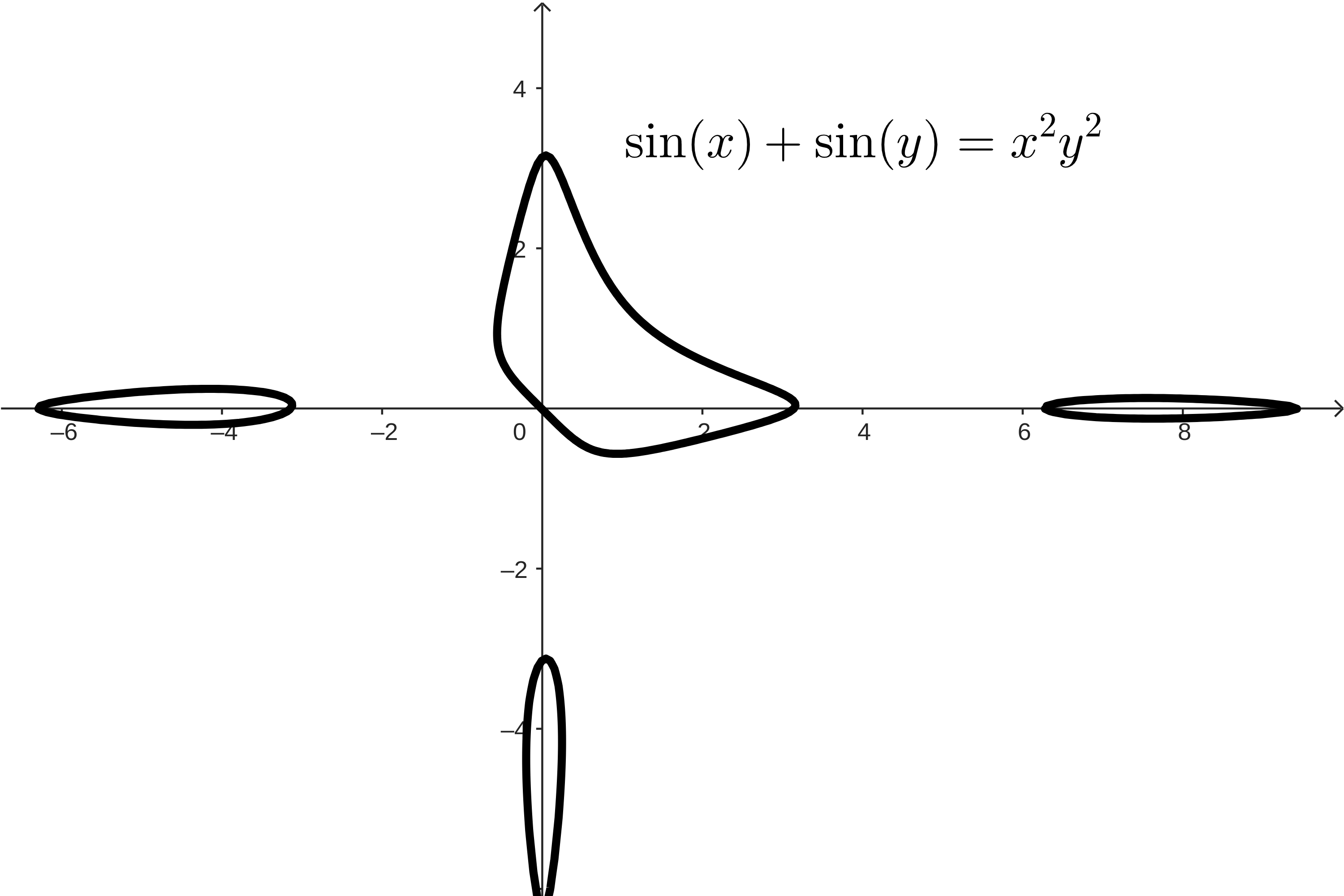
This curve is a special curve with some interesting mathematical properties, and is actually a part of a family of curves called elliptic curves. For now, let’s just consider it as a fun curve to look at, and use implicit differentiation to think about it.

🔗

The elliptic curve, y^2=x^3-x+1. If has a flared horseshoe type shape. The curve has a symmetry across the x-axis, and the upper section starts somewhere near (-1.3,0). It starts moving vertically upwards, and then curves towards (-1,1). From there, it descends lightly towards somewhere near (0.6, 0.6), where it flares upwards. The portion under the x-axis is a reflection of this. — Figure 3.1.3.
🔗

(a)

Mark the locations on the curve where it looks like the curve will have horizontal tangent lines. How many did you find?

🔗

(b)

Mark the locations on the curve where it looks like the curve will have vertical tangent lines. How many did you find?

🔗

(c)

Find the point(s) where \(x=0\text{.}\) What do you think the value of the derivative, \(\dydx\text{,}\) would be at these points?

🔗

(d)

For the elliptic curve defined by the equation \(y^2=x^3-x+1\text{,}\) apply the derivative to both sides of this equation:

\begin{align*} \ddx{y^2} \amp = \ddx{x^3-x+1}\\ \ddx{y^2} \amp = \ddx{x^3}-\ddx{x} + \ddx{1} \end{align*}

Carefully consider each of these derivatives (each of the terms). Which of these will you need to apply the Chain Rule for?

🔗

(e)

Differentiate. Solve for \(\dydx\) or \(y'\text{,}\) whichever notation you decide to use.

🔗

Hint 1.

Make sure to use the Chain Rule when necessary!

🔗

Hint 2.

\(\Ddx{y^2} = \Dd{}{y}\left(y^2\right)\Dydx = 2y\cdot \Dydx\) or \(2yy'\)

🔗

(f)

Go back to the first few questions, and try to answer them again:

Find the locations of any horizontal tangent lines (where \(\dydx=0\)).
🔗

🔗
Find the locations of any vertical tangent lines (where \(\dydx\) doesn’t exist, or where you would divide by 0).
🔗

🔗
Find the values of \(\dydx\) for the points on the curve where \(x=0\text{.}\)
🔗

🔗

🔗

This example was pretty similar to the first activity: in both of these, we use the Chain Rule to differentiate \(\ddx{y^2}\text{.}\) Let’s look at another example.

🔗

Activity 3.1.3. A New Curve.

Let’s consider a new curve:

\begin{equation*} \sin(x)+\sin(y)=x^2y^2\text{.} \end{equation*}

A curve with 4 independent loops visible. The main, middle, loop, looks like a deformed circle. It passes through the origin, and has some straight sides and almost pointed corners, although they are still round. On the x-axis, there are two very flat round loops: one around (8,0) and another around (-5,0). A third one lays on the y-axis around (-5,0). — Figure 3.1.4.
🔗

🔗

(a)

We are going to find \(\dydx\) or \(y'\text{.}\) Let’s dive into differentiation:

\begin{align*} \ddx{\sin(x)+\sin(y)} \amp =\ddx{x^2y^2}\\ \ddx{\sin(x)} + \ddx{\sin(y)} \amp = \ddx{x^2y^2} \end{align*}

Think carefully about these derivatives. For each of the three, how will you approach it? What kinds of nuances or rules or strategies will you need to think about? Why?

🔗

Hint.

Are any of these derivatives involving a variable other than \(x\text{,}\) the input variable (based on our \(\dydx\) notation, since we are thinking about how \(y\) changes with regard to \(x\)).

🔗

Are any of these derivatives involving any other combination of functions? Are there products and/or quotients that we need to think about?

🔗

(b)

Implement your ideas or strategies from above to differentiate each term.

🔗

Hint.

We need to apply the Chain Rule to \(\ddx{\sin(y)}\) and then we need to apply the Product Rule \(\ddx{x^2y^2}\text{.}\) Notice that when we find the derivative of \(y^2\) for the Product Rule, we need to use the Chain Rule!

🔗

Solution.

\begin{align*} \ddx{\sin(x)+\sin(y)} \amp =\ddx{x^2y^2}\\ \ddx{\sin(x)} + \ddx{\sin(y)} \amp = \ddx{x^2y^2}\\ \cos(x) + \cos(y)\cdot \dydx \amp = 2xy^2 + 2x^2y\cdot \dydx\\ \text{or } \cos(x)+y'\cos(y) \amp = 2xy^2 + 2x^2yy' \end{align*}

🔗

(c)

Now we need to solve for \(\dydx\) or \(y'\text{,}\) whichever you are using. While this equation can look complicated, we can notice something about the “location” of \(\dydx\) or \(y'\) in our equation.

🔗

Why do we always know that \(\dydx\) or \(y'\) will be multiplied on a term whenever it shows up?

🔗

(d)

Now that we are confident that we will always know that we are multiplying this derivative, we can employ a consistent strategy:

Rearrange our equation so that every term with a \(\dydx\) or \(y'\) is on one side, and everything without is on the other.
🔗

🔗
Now we are guaranteed that \(\dydx\) or \(y'\) is a common factor: factor it out.
🔗

🔗
Now we can solve for \(\dydx\) or \(y'\) by dividing!
🔗

🔗

Solve for \(\dydx\) or \(y'\) in your equation!

🔗

(e)

Build the equation of a line that lays tangent to the curve at the origin. Does the value of \(\dydx\) at \((0,0)\) look reasonable to you?

🔗

Subsection Some Summary and Strategy

Let’s wrap this up with some general strategy and summary of what we’ve seen.

🔗

The first thing we can notice is that we have talked through how to employ two of the three big derivative rules: we used the Chain Rule throughout these examples, and in Activity 3.1.3 we needed to use the Product Rule in order to differentiate \(\ddx{x^2y^2}\text{.}\) We have a glaring omission from our examples so far, though. Where is the Quotient Rule?

🔗

In these implicitly defined curves, we can manipulate the equations to never have to think about division! Consider the curve:

\begin{equation*} \frac{\sin(x)}{x} + \frac{\sin(y)}{x} = xy^2\text{.} \end{equation*}

Graph this curve in a graphing utility like Desmos. Does it look any different than the curve in Activity 3.1.3?

🔗

The only difference, really, is that the curve with the division is not defined at \(x=0\text{.}\) As long as we keep those domain issues in mind, we can multiply everything by \(x\) to get our familiar equation:

\begin{equation*} \sin(x)+\sin(y)=x^2y^2\text{.} \end{equation*}

And there we go, we never have to think about the Quotient Rule in these kinds of contexts!

🔗

So we really only need a strategy for using the Chain Rule and the Product Rule.

🔗

Strategy for Implicit Differentiation.

We use the Chain Rule whenever we differentiate something like \(\dd{}{y}\left(f(y)\right)\text{.}\) We differentiate whatever the function is, and multiply by the derivative of \(y\text{:}\) \(f'(y)y'\text{.}\)
🔗

This generalizes more: any time the variable in our derivative notation does not match the variable in the function/term, we need to use the Chain Rule:

\begin{equation*} \dd{}{y}\left(e^x\right) \hspace{0.7cm} \dd{}{t}\left(\sin(x)\right) \hspace{0.7cm} \dd{}{x}\left(y^4\right) \end{equation*}

🔗

🔗
We use the Product Rule whenever we differentiate a term with some combination of \(x\) and \(y\) variables. More generally, we can use the Product Rule any time we have a combination of at least two variables. We have to treat these as different kinds of functions getting multiplied!

\begin{equation*} \dd{}{y}\left(xe^y\right) \hspace{0.7cm} \dd{}{t}\left(\cos(t)\sin(x)\right) \hspace{0.7cm} \dd{}{x}\left(y^4\sqrt{x+1}\right) \end{equation*}

🔗

🔗

🔗

From here on out, we will use the ideas of implicit differentiation to accomplish two things:

We have a bit more flexibility with how we think of derivatives! We do not need to be restricted to only thinking about functions in order to think about rates of change or slopes at a point. We can think about any curve, any relationship between variables, and think about the relationship between them based on how one changes with regard to the other.
🔗

🔗
Implicit differentiation will be a very useful tool. Even when we have functions that can be written explicitly, they might be hard to deal with -- overly complex or maybe involving functions that we aren’t used to. It is absolutely possible, and a really useful strategy, to rewrite the relationship between variables implicitly! We can maybe create a version of these equations that we can differentiate!
🔗

🔗

We’re going to use this second idea first: in the next section we’ll be thinking about inverse functions. We do not have any idea of how to think about derivatives of logarithmic functions, like \(y=\ln(x)\text{.}\)

🔗

We can rewrite this:

\begin{equation*} y=\ln(x) \longleftrightarrow x=e^y\text{.} \end{equation*}

This second representation is something we can differentiate!

🔗

Similarly, if we wanted to think about the derivative of \(y=\tan^{-1}(x)\text{,}\) we might instead think about rewriting this:

\begin{equation*} y=\tan^{-1}(x) \longleftrightarrow x=\tan(y)\text{.} \end{equation*}

There are some weird issues to think about with the domains and ranges of these functions, but this is how we’ll approach these derivatives next.

🔗

Practice Problems Practice Problems

1.

Explain the difference between \(\ddx{x^2}\) and \(\ddx{y^2}\text{.}\) How is the differentiation process different in each? Why?

🔗

2.

Explain why we need to use the product rule to differentiate \(\ddx{ye^x}\text{.}\)

🔗

3.

Use implicit differentiation to find \(\dydx\) or \(y'\text{.}\) Make a note of when you are using the product or chain rule, and make sure you know why you are using them.

🔗

(a)

\(x^2-y^2 = 0\)

🔗

(b)

\(4x+\sin(y) = 0\)

🔗

(c)

\(ye^x + 1=0\)

🔗

(d)

\(x^3\tan(y) + e^y - 10x = 1\)

🔗

(e)

\(y^3 - xy = x^2 - 2x\)

🔗

(f)

\(4xy - y\sec(x) + x^5 = 0\)

🔗

(g)

\(\cos(xy)-x^3y^2=0\)

🔗

(h)

\(4x^3 = y^2(4-x)\)

🔗

4.

Pick 2 problems from Practice Problem 3, above, that you can solve for \(y\) explicitly. Find the derivative \(\dydx\) or \(y'\) this way, and confirm that your answers are the same.

🔗

5.

Pick 2 problems from Practice Problem 3, above, that you cannot solve for \(y\) explicitly. Explain why implicit differentiation is a useful method here.

🔗

6.

For the following curves, find the equation of the line tangent at the point given.

🔗

(a)

\(3x^3+7y^3=10y\) at the point \((1,1)\)

🔗

(b)

\(x^3+y^3=9xy\) at the point \((4,2)\)

🔗

(c)

\(y(x^2+4) = 8\) at the point \((0,2)\)

🔗

(d)

\((x^2+y^2)^2 = \dfrac{25}{4}xy^2\) at \((1,2)\)

🔗

7.

Find the locations of the horizontal and vertical tangent lines for the curve:

\begin{equation*} x^2+y^2+2xy = 12\text{.} \end{equation*}

🔗

8.

Consider the following curve:

\begin{equation*} (xt+1)^3=t-x^2+7\text{.} \end{equation*}

🔗

(a)

Find \(\frac{dx}{dt}\text{.}\) Explain where you need to use the chain rule and why.

🔗

(b)

Find \(\frac{dt}{dx}\text{.}\) Explain where you need to use the chain rule and why.

🔗

Related Rates.

The rest of the exercises are related rates problems.

🔗

9.

Consider the equation:

\begin{equation*} 3r + 5y^2 - 4 = 3\sin(x)\text{.} \end{equation*}

Differentiate both sides with regard to the variable \(t\text{,}\) and solve for \(\frac{dr}{dt}\text{.}\)

🔗

10.

Consider the equation:

\begin{equation*} 3r + 5y^2 - 4 = 3\sin(x)\text{.} \end{equation*}

Differentiate both sides with regard to the variable \(t\text{,}\) and solve for \(\frac{dy}{dt}\text{.}\)

🔗

11.

A crab is walking along a path defined by the parabola \(y=x^2+1\text{.}\) It moves horizontally forward at a rate of 2 units/second, \(\frac{dx}{dt}=2\text{.}\) If it is currently at the point \((2,5)\text{,}\) what is the crab’s vertical speed, \(\frac{dy}{dt}\text{?}\)

🔗

12.

Person A is holding a balloon 30m away from another Person B. If the balloon is released and floats into the air, rising straight up at a speed of 0.5m/s. Person B watches the balloon, their eye-line forming an angle \(\theta\) with the ground. When the balloon is 10m up in the air, what is the speed at which \(\theta\) changes, \(\frac{d\theta}{dt}\text{?}\)

🔗

13.

A paper cup shaped like a cone is leaking water out of the bottom. The cup is 4 inches tall, and the radius is 1/3 of the height. If the water is leaking at a rate of 1.5 in\(^3\)/s while the the cup is full, how quickly is the height of the water in the cup decreasing?

🔗

14.

A 12 foot ladder is leaning against a vertical wall. Someone is pushing the base of the ladder closer to the wall at a speed of 0.5 ft/s. If the ladder is currently 6 feet away from the wall, how quickly does the top of the ladder move up the wall?

🔗

15.

A spherical water balloon is leaking water. The radius of the balloon is currently 2 inches, and we notice that it is decreasing at a rate of 1 in/min. How fast is the water leaking, in in\(^3\)/min?

🔗

Prev Top Next