We’re going to stick with our theme of thinking about a Riemann Sum, but this time we’ll get back to thinking about area. First, we’ll try to remind ourselves not just of what a Riemann sum is, but how we actually constructed it.
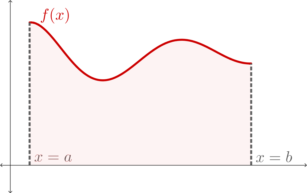
Let’s start with the function \(f(x)\) on the interval \([a,b]\) with \(f(x) \gt 0\) on the interval. We will construct a Riemman sum to approximate the area under the curve on this interval, and then build that into the integral formula.
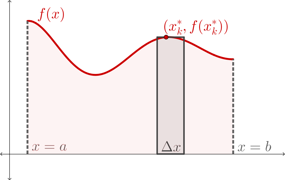
Pick an \(x_k^*\) for \(k=1,2,3,4\text{,}\) one for each subinterval. Then, plot the points \((x_1^*, f(x_1^*))\text{,}\)\((x_2^*, f(x_2^*))\text{,}\)\((x_3^*, f(x_3^*))\text{,}\) and \((x_4^*, f(x_4^*))\text{.}\)
These points are just general ones, and you don’t have to come up with actual numbers for the \(x\)-values or the corresponding \(y\)-values. Instead, just draw them in on the curve, somewhere in each of the subintervals.
You won’t have any numbers to calculate here, really: instead, see if you can calculate the widths by thinking about the total width of your interval. Then calculate the heights by thinking about the points you created.
Try to think about the accuracy of your area approximation by looking at it visually. Are there any places where your approximation looks far away from the actual area we’re thinking about?
Now we will generalize a little more. Let’s say we divide this up into \(n\) equally-sized pieces (instead of 4). Instead of trying to pick an \(x_k^*\) for the unknown number of subintervals (since we don’t have a value for \(n\) yet), let’s just focus on one of these: the arbitrary \(k\)th subinterval.
Apply a limit as \(n\to \infty\) to this Riemann sum in order to construct the integral formula for the area under the curve \(f(x)\) from \(x=a\) to \(x=b\text{.}\)
Hopefully this is helpful. If you’d like more reminders on this, you can always revisit Section 5.2 Riemann Sums and Area Approximations. For now, though, we mainly want to think about the general process we’re using:
We slice the region from \(x=a\) to \(x=b\) into \(n\) pieces, and, for convenience, we choose an equal width: \(\Delta x = \frac{b-a}{n}\text{.}\)
From each of the slices, we select some \(x\)-value (called \(x_k^*\) from the \(k\)th slice). We use that to evaluate the function on each slice: \(f(x_k^*)\text{.}\)
We multiply the function value, \(f(x_k^*)\text{,}\) by the width of the slice, \(\Delta x\text{,}\) to get the measured area of each slice, \(A_k = f(x_k^*)\Delta x\text{.}\)
We’re going to use this process (we’ll call it the slice-and-sum process) for other measurements! Let’s see how we can change this slightly to measure a different area.
SubsectionBuilding an Integral Formula for the Area Between Curves
Activity6.2.2.Area Between Curves.
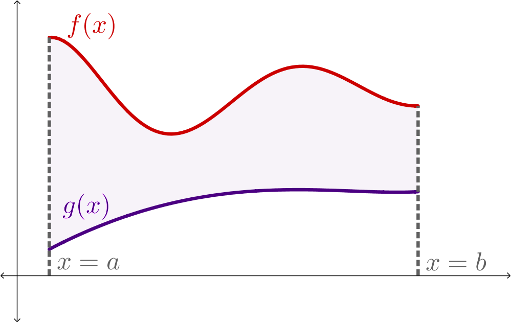
Let’s start with our same function \(f(x)\) on the same interval \([a,b]\)m but also add the function \(g(x)\) on the same interval, with \(f(x) \gt g(x) \gt 0\) on the interval. We will construct a Riemann sum to approximate the area between these two curves on this interval, and then build that into the integral formula.
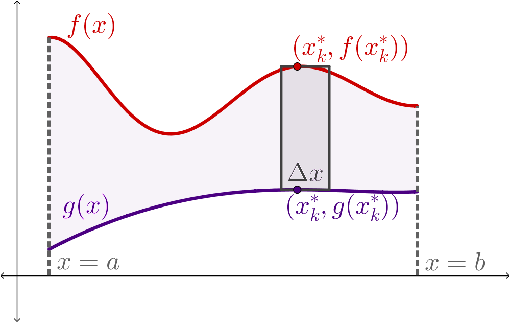
Pick an \(x_k^*\) for \(k=1,2,3,4\text{,}\) one for each subinterval. Plot the points \((x_1^*, f(x_1^*))\text{,}\)\((x_2^*, f(x_2^*))\text{,}\)\((x_3^*, f(x_3^*))\text{,}\) and \((x_4^*, f(x_4^*))\text{.}\) Then plot the corresponding points on the \(g\) function: \((x_1^*, g(x_1^*))\text{,}\)\((x_2^*, g(x_2^*))\text{,}\)\((x_3^*, g(x_3^*))\text{,}\) and \((x_4^*, g(x_4^*))\text{.}\)
Use these 8 points to draw 4 rectangles, with the points on the \(f\) function defining the tops of the rectangles and the points on the \(g\) function defining the bottoms of the rectangles. What are the dimensions of these rectangles (the height and width)?
Now we will generalize a little more. Let’s say we divide this up into \(n\) equally-sized pieces (instead of 4). Instead of trying to pick an \(x_k^*\) for the unknown number of subintervals (since we don’t have a value for \(n\) yet), let’s just focus on one of these: the arbitrary \(k\)th subinterval.
Apply a limit as \(n\to \infty\) to this Riemann sum in order to construct the integral formula for the area between the curves \(f(x)\) and \(g(x)\) from \(x=a\) to \(x=b\text{.}\)
If \(f(x)\) and \(g(x)\) are continuous functions with \(f(x)\geq g(x)\) on the interval \([a,b]\text{,}\) then the area bounded between the curves \(y=f(x)\) and \(y=g(x)\) between \(x=a\) and \(x=b\) is
\begin{equation*}
A = \int_{x=a}^{x=b} \left(f(x)-g(x)\right)\;dx\text{.}
\end{equation*}
When we’re applying this formula for the area between curves, we won’t need to recreate the process from Activity 6.2.2 to create the integral formula. We simply can identify the functions bounding the region and the end points of the interval, and set up the integral.
We’ll use the slice-and-sum process for two reasons:
To justify these formulas that we continue to build! While this one isn’t that difficult (you could have just built the formula by thinking about the area between curves as a difference in areas under each curves), some of the formulas we play with in this chapter will not be as intuitive.
To help us understand what a Riemann sum actually is. It’s a product of a function value from a subinterval multiplied by the width of that subinterval, summed up across some larger interval.
For each of the following regions, set up an integral expression representing the area of the region. We also can practice evaluating these integrals to actually calculate the areas.
For each of these described regions, the hint will reveal a visualization of the region (using Desmos). Feel free to use that to set up the integral expression!
Notice that the boundary functions intersect at \(x=\frac{\pi}{4}\text{,}\) and they switch order. We’ll need to split this region into two different regions in order to identify the "top" and "bottom" boundary functions.
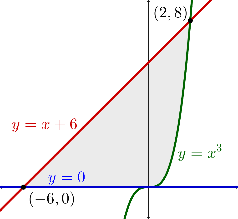
On the interval \(-6\leq x\leq 0\text{,}\) the region is bounded above by \(y=x+6\) and below by the \(x\)-axis (\(y=0\)). On the interval \(0\leq x\leq 2\text{,}\) the region is bounded above by \(y=x+6\) and below by \(y=x^3\text{.}\)
This last example had two interesting regions: we had to split them into two pieces because the boundary functions changed order or, in the case of the last example, changed completely to different boundary functions.
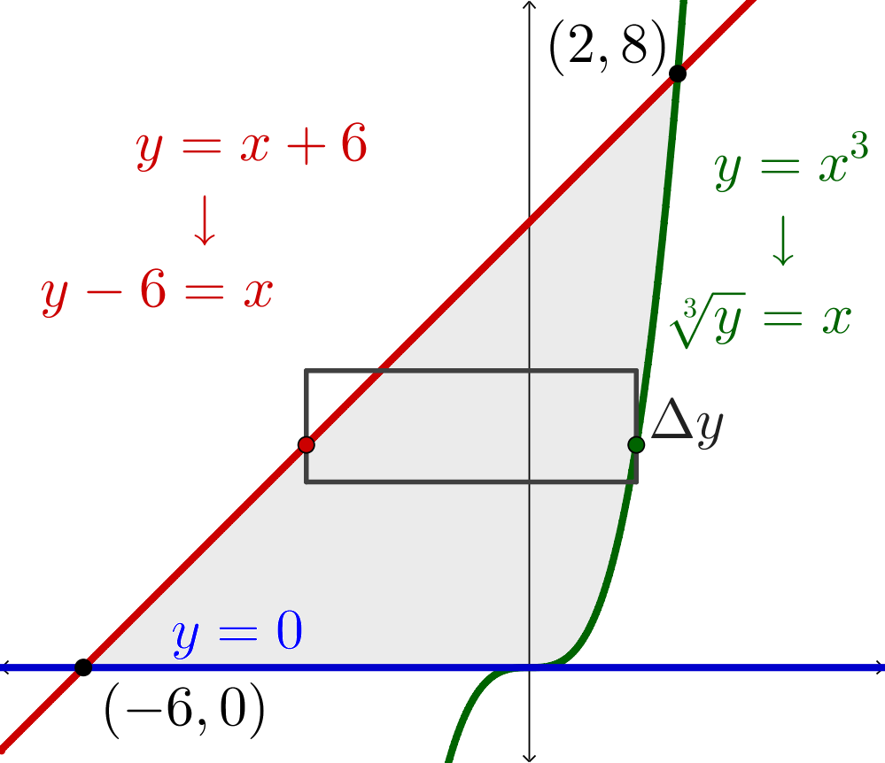
Let’s consider the same setup as earlier: the region bounded between two curves, \(y=x+6\) and \(y=x^3\text{,}\) as well as the \(x\)-axis (the line \(y=0\)). We’ll need to name these functions, so let’s call them \(f(x) = x^3\) and \(g(x) = x+6\text{.}\) But this time, we’ll approach the region a bit differently: we’re going to try to find the area of the region using only a single integral.
The range of \(y\)-values in this region span from \(y=0\) to \(y=8\text{.}\) Divide this interval evenly into 4 equally sized-subintervals. What is the height of each subinterval? We’ll call this \(\Delta y\text{.}\)
Find the corresponding \(x\)-values on the \(f(x)\) function for each of the \(y\)-values you selected. These will be \(f^{-1}(y_1^*)\text{,}\)\(f^{-1}(y_2^*)\text{,}\)\(f^{-1}(y_3^*)\text{,}\) and \(f^{-1}(y_4^*)\text{.}\)
You’re really just putting your \(y\)-values into the equation \(y=x+6\) and solving for \(x\text{.}\) Or you can solve for \(f^{-1}(y)\) in general, by solving for \(x\) while leaving \(y\) as a variable.
Do the same thing for the \(g\) function. Now you have 8 points that you can plot: \(\left(f^{-1}(y_1^*), y_1^*\right)\text{,}\)\(\left(f^{-1}(y_2^*), y_2^*\right)\text{,}\)\(\left(f^{-1}(y_3^*), y_3^*\right)\text{,}\) and \(\left(f^{-1}(y_4^*), y_4^*\right)\) as well as \(\left(g^{-1}(y_1^*), y_1^*\right)\text{,}\)\(\left(g^{-1}(y_2^*), y_2^*\right)\text{,}\)\(\left(g^{-1}(y_3^*), y_3^*\right)\text{,}\) and \(\left(g^{-1}(y_4^*), y_4^*\right)\text{.}\) Plot them.
Use these points to draw 4 rectangles with points on \(f\) and \(g\text{,}\) determining the left and right ends of the rectangle. What are the dimensions of these rectangles (height and width)?
Which variable defines the location of the \(k\)th rectangle, here? That is, if you were to describe where in this graph the \(k\)th rectangle is laying, would you describe it with an \(x\) or \(y\) variable? This will act as our general input variable for the integral we’re ending with.
Apply a limit as \(n\to \infty\) to this Riemann sum in order to construct the integral formula for the area between the curves \(f(x)\) and \(g(x)\) from \(x=a\) to \(x=b\text{.}\)
Now that you have an integral, evaluate it! Find the area of this region to compare with the work we did previously, where we used multiple integrals to measure the size of this same region.
We can rewrite our definition of the area between curves (Definition 6.2.5) to account for this change in perspective, by thinking about these same functions in terms of \(y\text{.}\)
Definition6.2.9.Area Between Curves (in terms of \(y\)).
If \(f(y)\) and \(g(y)\) are continuous functions with \(f(y) \geq g(y)\) on the interval of \(y\)-values \([c,d]\text{,}\) then the area bounded between the curves \(x=f(y)\) and \(x=g(y)\) from \(y=c\) to \(y=d\) is
\begin{equation*}
A = \int_{y=c}^{y=d} \left( f(y) - g(y)\right)\;dy\text{.}
\end{equation*}
This strategy of inverting our functions to change the variable that we integrate with regard to is useful, but a tricky part of this is deciding when to change variables.
Something that we can look for is intersection points in the region we’re working with. If, in our plan for setting up an integral, we would stack rectangles that would pass through an intersection point, then this indicates that we would need to split our region up to set up the integrals (since the boundary functions are changing). If we change the orientation of the rectangles, would they still pass through an intersection point? Are the functions that we’re working with relatively easy to invert? Can we antidifferentiate these functions, or their inverted versions?
To finish things up, let’s look at a nice little interactive graph that can help show the differences between finding area with regard to \(x\) (using \(\Delta x\) in our rectangles and \(dx\) in our integrals) and finding area with regard to \(y\) (using \(\Delta y\) in our rectangles and \(dy\) in our integrals).
Explain how we use the "slice and sum" method to build an integral formula for the area bounded between curves. Give some details, enough to make sure you understand how the Riemann sums are constructed and how they turn into our integral formula.
Set up and evaluate an integral representing the area of each of the regions described below. Explain whether you chose to integrate with respect to \(x\) or \(y\text{,}\) and why you made that choice.