Before we move on to our actual goal of analyzing infinite series, we will construct infinite sequences. The big thing to remember here is that, when we build and analyze these sequences, we are are really building and analyzing functions. We want to keep this idea of sequences as functions in the forefront, since it will help us as we think about accumulating these function values into infinite series.
We might already have some familiarity with sequences. Here, we’ll focus less on some of the detailed mechanics and just think about these sequences as functions.
Describe a sequence of numbers where you use a consistent rule/function to build each term (each number) based only on the previous term in the sequence. You will need to decide on some first term to start your sequence.
Describe a different sequence of numbers using the same rule to generate new terms/numbers from the previous one. What do you need to do to make these two sequences different from each other?
Describe a new sequence of numbers where you use a consistent rule/function to build each term based on its position in the sequence (i.e. the first term will be some rule/function based on the input 1, the second will be based on 2, you’ll use 3 to get the third term, etc.). We will call the position of each term in the sequence the index.
Describe another, new, sequence of numbers where you use a consistent rule/function to build each term based on its index. This time, make the terms get smaller in size as the index increases.
An infinite sequence defined using an explicit formula is one where the \(k\)th term of the sequence is defined as a function output of \(k\text{,}\) the term’s index.
A sequence is defined using a recursion relation is one where the \(k\)th term of the sequence is defined as a function output of the previous term, the \((k-1)\)st term. The sequence also needs some initial term to base the subsequent terms from.
These definitions are relatively limited. You might, for instance, know of a very famous sequence that is defined recursively by having each term being the sum of the two previous terms. Our study of sequences will be brief and will be leading us towards infinite series, so there are a lot of nuances about sequences that we will skip.
Now, for each sequence, define the sequence formally using either an explicit formula or recursion relation, whichever matches with how you described the sequence in Activity 8.1.1.
For each of the following sequences, write out the first handful of terms. There isn’t a set amount, but you should write out enough to get a feel for the sequence structure and how the different ways of defining the sequences work. In each, you can start the index \(k\) at 1 and count upwards (\(k=1,2,3,...\)).
If you’re not sure, maybe you need to write out a few more terms! You can also change how you write the numbers themselves: in some cases, fractions might be helpful, but in others it might be useful to write the numbers in decimal form. Maybe you’ll approximate values of the sine or exponential functions, or maybe you’ll leave them as \(\sin(2)\) or \(e^3\text{.}\)
Some of these limits, as \(k\to \infty\text{,}\) will be tricky to work with! When might you want to use The Squeeze Theorem? When might you want to use L’Hôpital’s Rule?
We’ll look at some sequences by writing out the first handful of terms. From there, our goal is to write out more terms and eventually define each sequence fully.
For each sequence, write an explicit formula and a recursion relation to define the sequence. You can choose whether to start your index at \(k=0\) or \(k=1\text{.}\)
It might be helpful to write these numbers using a common denominator! Or at least some of the numbers. Alternatively, you can try a common numerator (which is very fun to do, since we normally don’t do that).
If you are recursively multiplying by a number each time, what will that look like in the explicit formula? How do we represent repeated multiplication?
Rewrite \(\frac{2}{5}\) and \(\frac{3}{13}\) by scaling the numerator and denominator by 2. Can you find a formula for the numerator and denominator separately? This one is very difficult to find a recursion relation for, so feel free to only write it explicitly!
Before moving on, we should make a couple of notes:
When we add something recursively (where we add the same thing repetitively to get from the \(k\)th term to the \((k+1)\)st term), this is the same thing as multiplication in an explicit formula!
In general, it can be pretty difficult to find either of these formulas for a given sequence of numbers. In fact, in any sequence where only the first few terms are given, we can find an infinite number of formulas that provide those first few terms and then deviate to any other numbers. We cannot easily extrapolate onto only one “pattern” or formula. Because of this, we’ll try to limit our work as much as we can to situations where we have the formula defining the sequences.
We have tried introducing and talking about sequences as special types of functions, mapping natural number inputs to real number outputs. If we are committed to thinking about sequences as functions, with maybe some special context, then we should really investigate how one of our primary representations of functions (graphs) manifests itself in this new context.
There really is not too much to think about here! We can focus on the domain of these functions. If we define a sequence \(\{a_k\}\) explicitly, then we have some function \(a_k = f(k)\text{,}\) and we can plot this sequence function in the same way that we normally would any other function \(g(x)\text{.}\) We will use the horizontal axis for the inputs and the vertical axis to represent the outputs, and try to visualize the graph as the set of all of the pairs of inputs with their (single) corresponding output.
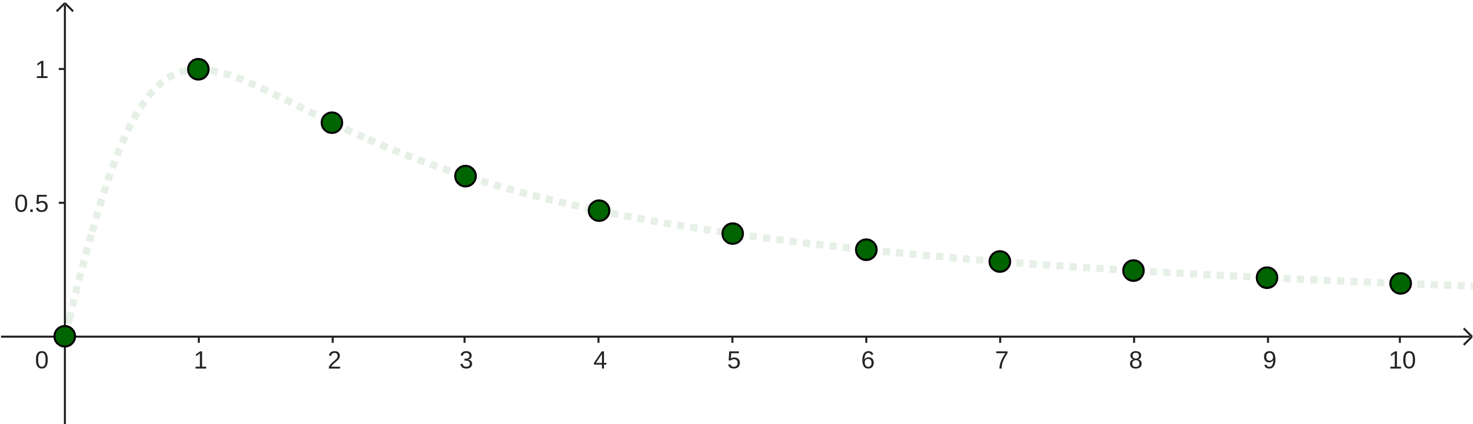
The only new feature, then, is that these functions have only non-negative integer inputs. So when we plot the points, we do not get some nice curve acting as a visual representation of the function: we get discrete points floating on the 2-dimensional plane, each with some consistent horizontal spacing between them.
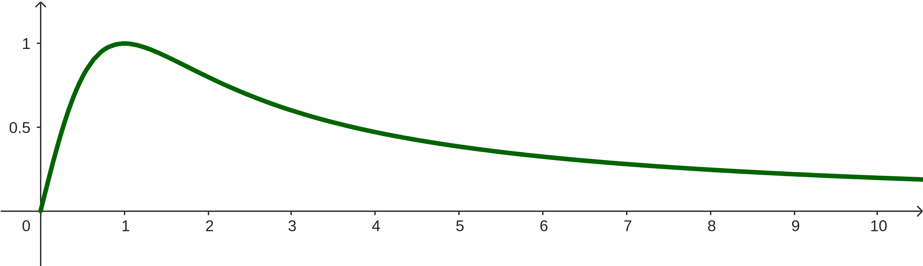
We will typically not plot these with the smooth curve of the corresponding continuous function plotted, but in this first example it is useful to highlight how we think about this sequence as a function.
Let’s continue to think about these sequences as just functions in a special kind of context. How does this discrete context change how we talk about functions and what kinds of terminology we use?
If a sequence is a function (and we’re saying in this introductory section that it is), then we can think of all of the different terminology and adjectives that we use to describe functions. How many of them are relevant to sequences?
We say that a sequence \(\{a_k\}_{k=1}^\infty\) is increasing if, for all \(k=1,2,3...\text{,}\)\(a_{k+1}\gt a_k\text{.}\) If \(a_{k+1}\geq a_k\) for all \(k=1,2,3,...\) then we say that \(\{a_k\}\) is non-decreasing.
We say that a sequence \(\{a_k\}_{k=1}^\infty\) is decreasing if, for all \(k=1,2,3...\text{,}\)\(a_{k+1}\lt a_k\text{.}\) If \(a_{k+1}\leq a_k\) for all \(k=1,2,3,...\) then we say that \(\{a_k\}\) is non-increasing.
We say that \(a_k\) is constant if \(a_{k+1}=a_k\text{,}\) but this is a very boring sequence and we will likely not think terribly hard about these kinds of sequences.
Sometimes we might say that a sequence is eventually decreasing (or eventually non-increasing) if there is some \(K\gt1\text{,}\) and the sequence is decreasing (or non-increasing) for \(k=K, K+1, K+2, ...\text{,}\) and similarly for eventually increasing or eventually non-decreasing.
A good example of a sequence that is eventually decreasing is the one we plotted in Figure 8.1.5. We can see that the sequence increases from \(k=0\) to \(k=1\) (since \(a_0\lt a_1\)), but then decreases after that.
We could think about the corresponding continuous function (the one plotted in Figure 8.1.5) and find the point at which our function starts decreasing: we just need to refer back to Theorem 4.2.6 First Derivative Test to find the interval(s) for which \(f(x)=\dfrac{x}{x^2+1}\) decreases.
We say that a sequence \(\{a_k\}_{k=1}^\infty\) is bounded below if there is some real number \(M\) such that \(a_k\geq M\) for all \(k=1,2,3,...\text{.}\)
Similarly we say that a sequence \(\{a_k\}_{k=1}^\infty\) is bounded above if there is some real number \(N\) such that \(a_k\leq N\) for all \(k=1,2,3,...\text{.}\)
Lastly, we’ll focus on the end-behavior of a sequence. We’ll think about convergence of a sequence in the same way that we did for Improper Integrals: does the limit exist?
For the sequence \(\{a_k\}\text{,}\) if \(L\) is some real number and \(\lim_{k\to\infty}a_k = L\text{,}\) the we say that the sequence \(\{a_k\}\) converges to \(L\text{.}\) If this limit does not exist, we say that the sequence \(\{a_k\}\) diverges.
This theorem seems to be a bit obvious to many students: why would we care about this, when we can just find a limit of the explicit formula for a sequence? We’ll see throughout the rest of this chapter that this theorem is one of the most important and most useful results in our study of infinite sequences and infinite series. For now, though, let’s use it to find the limits of some recursively defined sequences.
Let’s revisit one of the recursively defined sequences that we’ve seen already and then think about a couple of other interesting ones. Before we do that, though, we should recognize why we need to treat recursively defined sequences a bit differently than ones defined explicitly.
In an explicit formula, the terms themselves are a function of \(k\text{,}\) the index. This means that we can simply apply a limit as \(k\to\infty\) to understand whether or not the sequence converges and what it might converge to. These limits could be tricky, but we have the tools to evaluate them! In a recursion relation, though, each term is not a function of the index, which means we can’t easily apply a limit as \(k\to\infty\) to the term definition.
We’ll be able to apply a limit, but it will feel a bit different: we’re going to go into the computational work for the limit already assuming that the limit exists. Let’s see how it goes.
What would this \(L\) be, if it exists? A key thing to note is that if \(\lim_{k\to\infty} a_k\) exists (and we have a symbol, \(L\text{,}\) for it) then we can say that
Whether or not this is obvious to you is not a mark of your understanding, but we need to make sure that this ends up being obvious to you. If it’s not, that’s ok! But it is an indicator that you should take a couple of minutes to think about this. Once you are convinced that these two limits are the same thing, move on to the next part.
And so we have two solutions to this equation: \(L=0\) and \(L=\frac{1}{2}\text{.}\) This is strange: how can a sequence have more than one value that it converges to?
It’s because we have yet to take into account the initial term, \(a_1\text{!}\) Depending on this value, the sequence might converge or not, and if it does converge, then there are two options for what the sequence can converge to, based on the value of \(a_1\text{.}\)
You can do the next part on your own, but I want you to pick different numbers for \(a_1\) and write out some terms of the resulting sequence. You should find that some of them look like they’re converging to \(0\text{,}\) one of them will converge to \(\frac{1}{2}\) (it’s a fun hunt to find which one), and some will diverge.
You should find that if \(a_1=\frac{1}{2}\text{,}\) then the sequence is constant and converges to \(\frac{1}{2}\text{.}\) If \(0\leq|a_1|\lt \frac{1}{2}\) then the sequence seems like it’ll converge to \(0\text{.}\) And if \(|a_1|\gt \frac{1}{2}\text{,}\) then it looks like the sequence diverges.
Now it is up to us to show that this sequence, with \(a_1 = \frac{1}{3}\text{,}\) does converge. Sure, we have some evidence and a good conjecture that it converges to \(\frac{1}{2}\text{,}\) but that is just our good guess based on what we have seen in the first handful of numbers.
It should be clear that \(a_k\gt 0\text{,}\) since as long as \(a_{k-1} \neq 0\text{,}\) then \((a_{k-1})^2\gt 0\text{.}\) Since we start with \(a_1 \neq 0\text{,}\) we are guaranteed to get non-zero values from the formula for a new term! Great news, we have a lower bound.
So the sequence \(\{a_k\}\) is bounded. Now we just need to convince ourselves that this sequence is monotonic. We know that our terms are bounded above by \(\frac{1}{2}\text{,}\) and I hope that this means we can convince ourselves that since our terms are smaller than this, which would produce a constant sequence, then all of our terms are probably decreasing.
We can solve for when this is negative! It shouldn’t be hard to show that \(a_k(2a_k-1)\lt 0\) when \(0\lt a_k \lt \frac{1}{2}\text{.}\) And we’ve already shown this is true in our case!
So \(\{a_k\}\) is bounded and monotonic and must therefore converge because of the Monotone Convergence Theorem. Because \(a_1\lt\frac{1}{2}\text{,}\) we know that this sequence doesn’t converge to \(\frac{1}{2}\text{,}\) and so must converge to the only other option: 0.
There are some other fun ways of doing this same thing for other recursive examples. The argument above is relatively bulky to use, and so we understandably will not think about recursively defined sequences very much: we’ll leave that topic for another course where we have more time to really explore them. If you are interested in trying this same argument with other sequences though, we’ll end this section with two more fun examples.
Write out some terms to get a feel for things! Then, assuming that the sequence converges to some real number, \(L\text{,}\) think about what happens when you apply a limit as \(k\to\infty\text{:}\) we should get the equation \(L=\sqrt{2+L}\text{.}\)
Write out some terms to get a feel for things! Then, assuming that the sequence converges to some real number, \(L\text{,}\) think about what happens when you apply a limit as \(k\to\infty\text{:}\) we should get the equation \(L=\frac{1}{2L+1}\text{.}\)
For each of the following sequences, write down a possibility for an explicit formula defining the sequence as well as a recursion relation (with initial value) defining the sequence.
Compare a sequence to a function. What are some similarities? What are some differences? Carefully discuss this in terms of different representations of sequences/functions.