
Section 4.2 Increasing and Decreasing Functions

Activity 4.2.1. How Should We Think About Direction?

Our goal in this activity is to motivate some new terminology and results that will help us talk about the “direction” of a function and some interesting points on a function (related to the direction of a function). For us to do this, we’ll look at some different examples of functions and try to think about some unifying ideas.
A rational function that increases gently up to a point in the third quadrant, then decreases towards a vertical asymptote at x=0. In the first quadrant, the function decreases down to some point, and then gently increases.
A polynomial function that decreases down to a point, then increases, then decreases, then increases.
A kind of oscillating function that looks like it bounces off of the horizontal axis, creating sharp corners. It gently changes direction near the peak. The graph decreases, hits the axis and increases, then gently decreases towards the horizontal axis. It bounces one more time, and increases then decreases.
A bell curve, with horizontal asymptote at y=0. It increases up to a point on the top where it changes to decreasing towards the horizontal axis.
Figure 4.2.1.
These examples do not cover all of the possibilities of how a function can act, but will hopefully provide us enough fertile ground to think about some different situations.
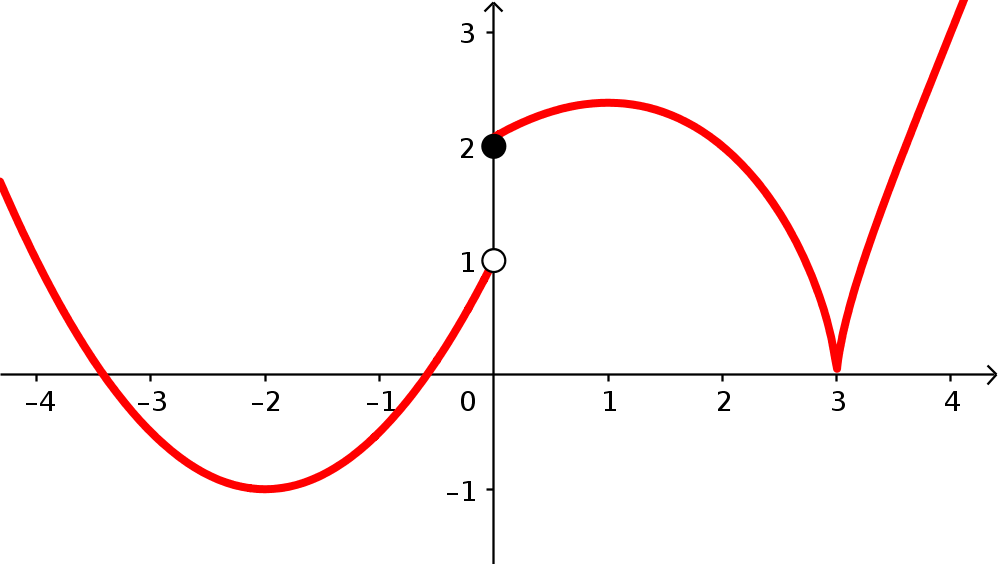
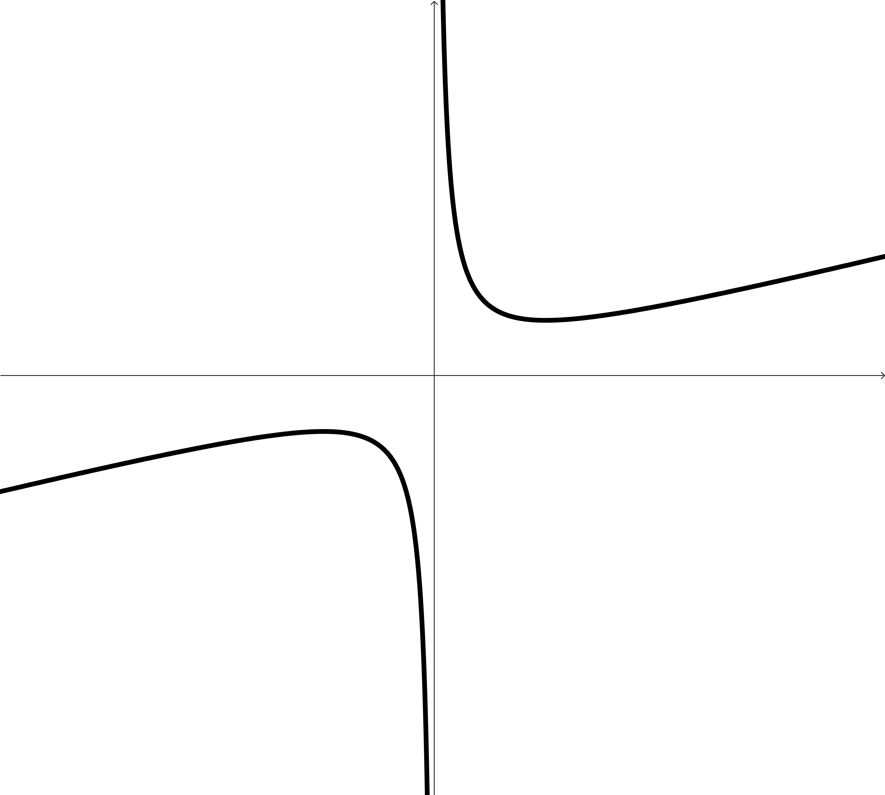
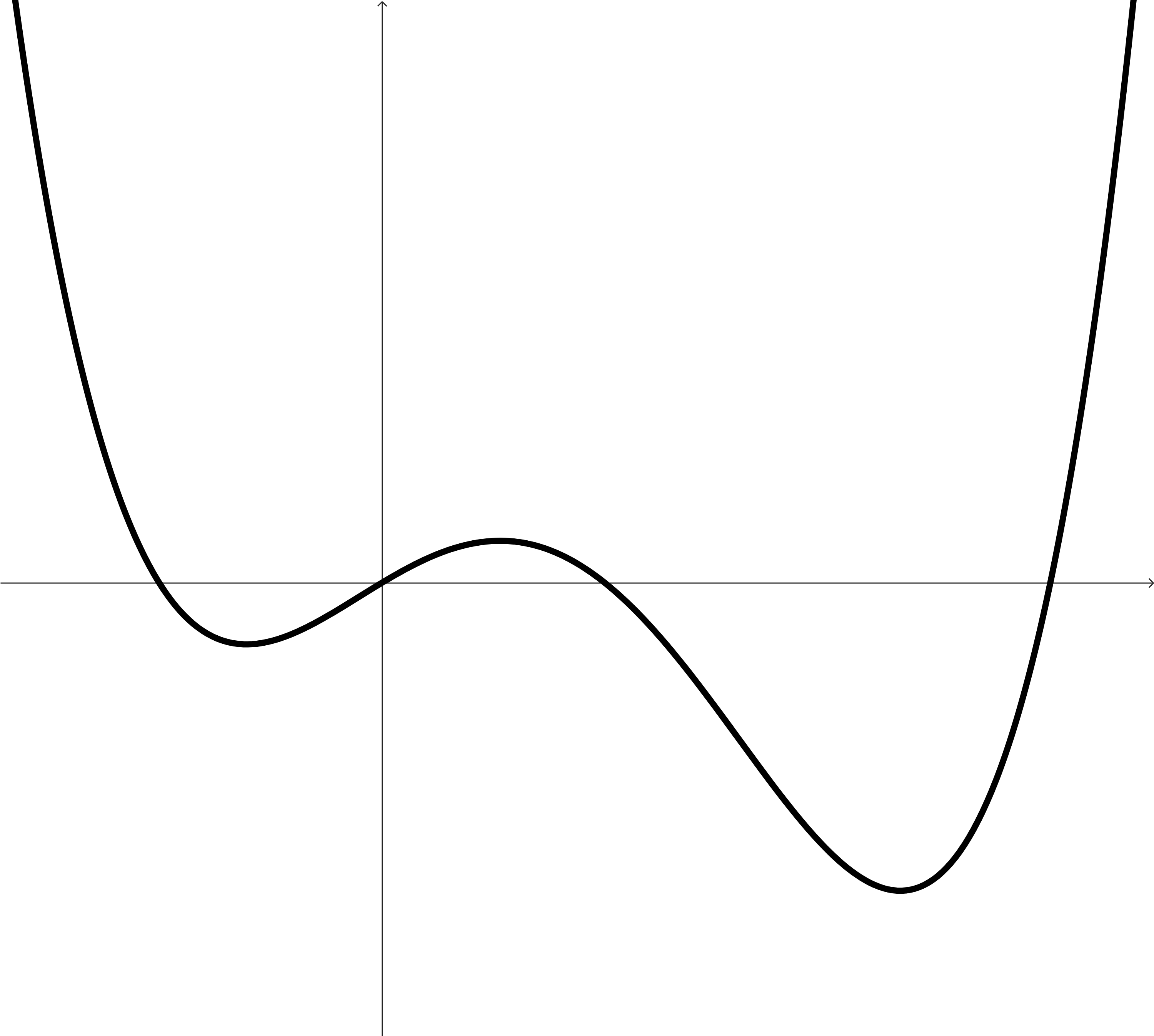
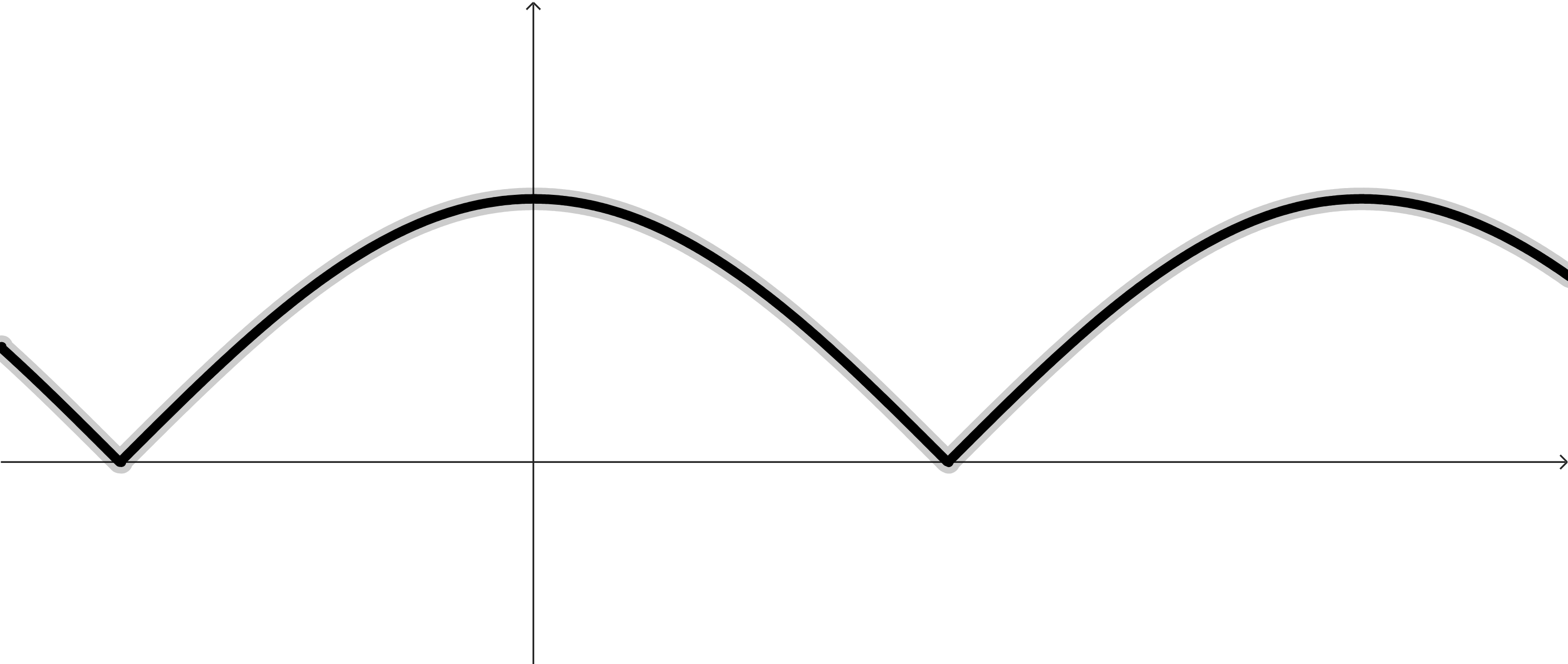
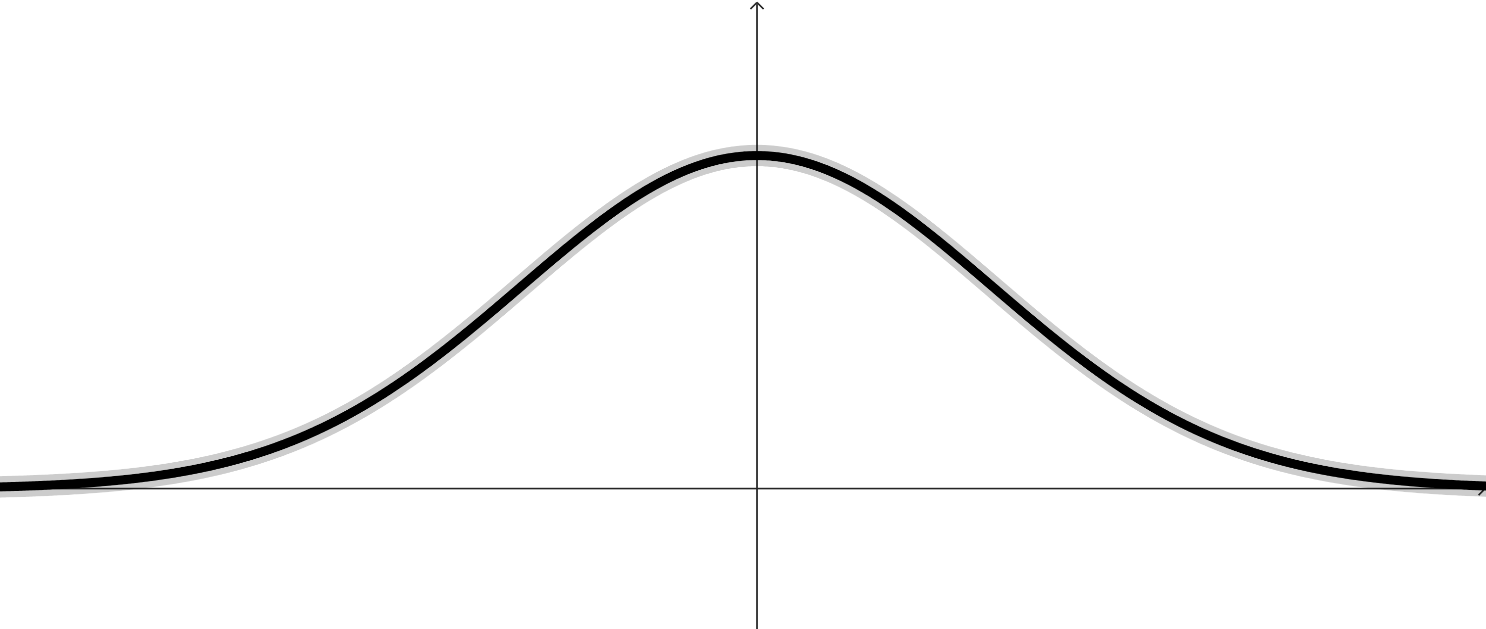
(a)

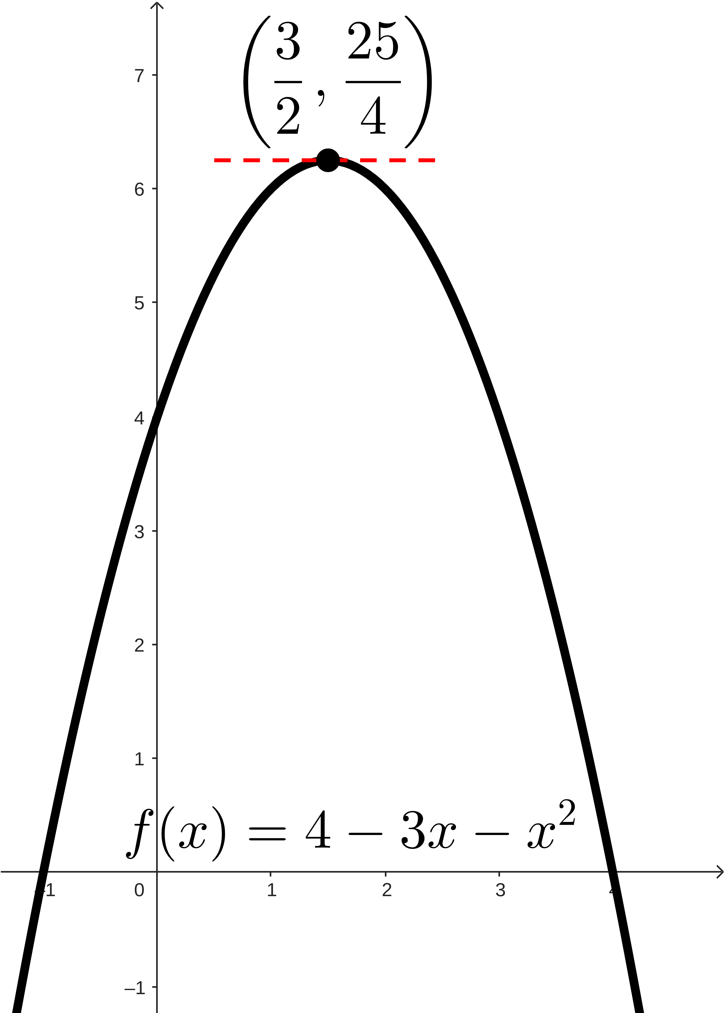
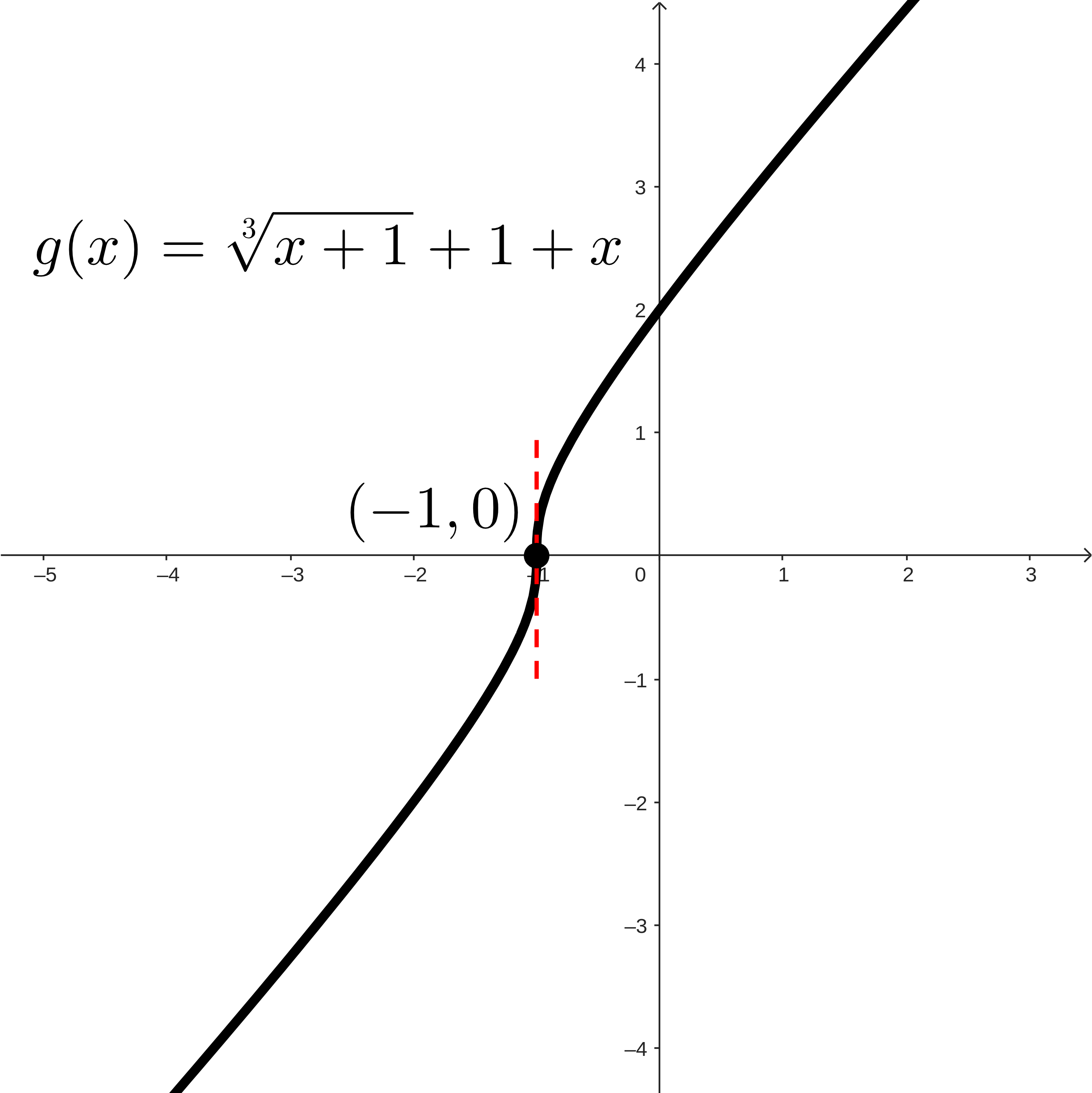
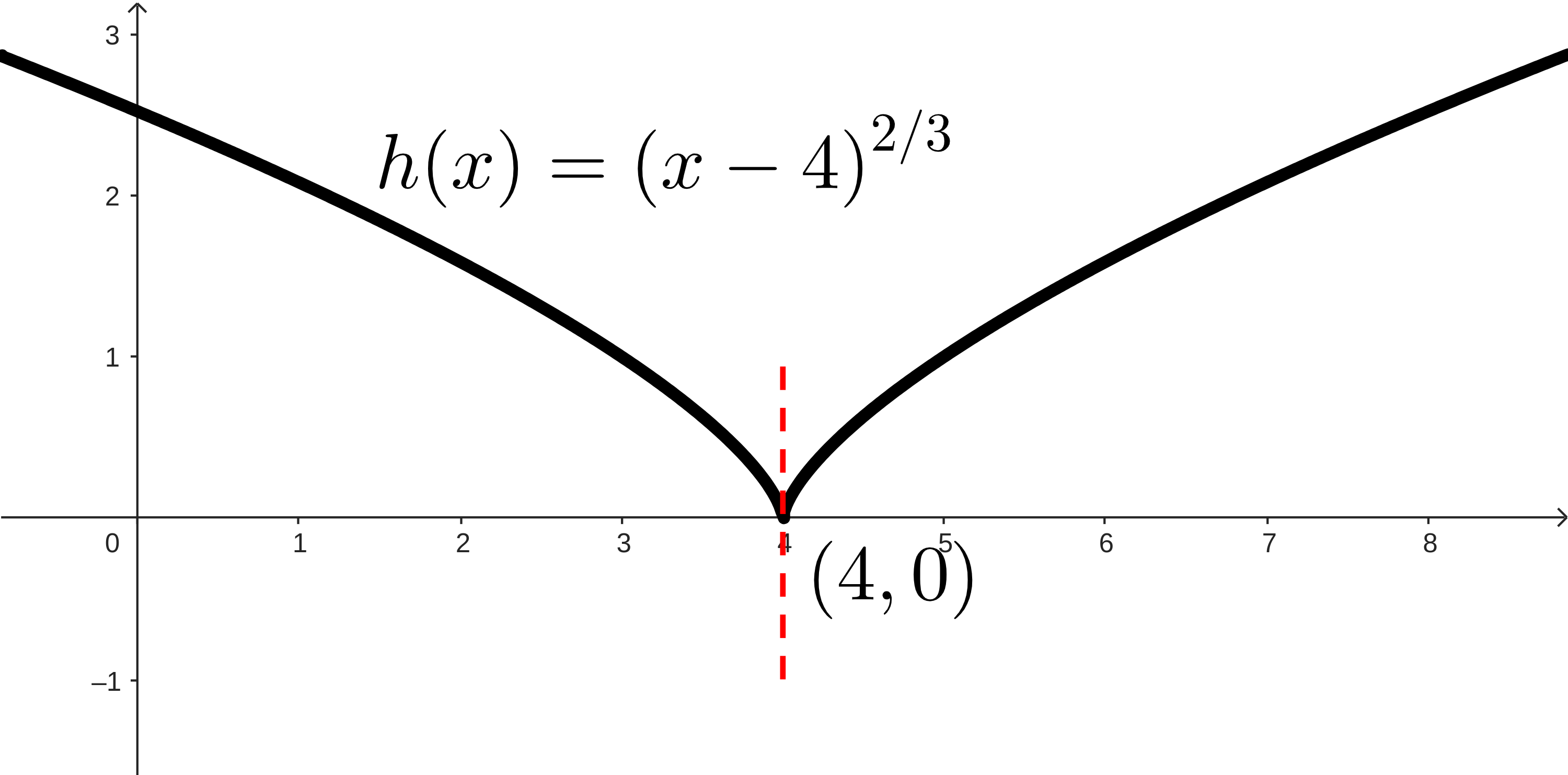
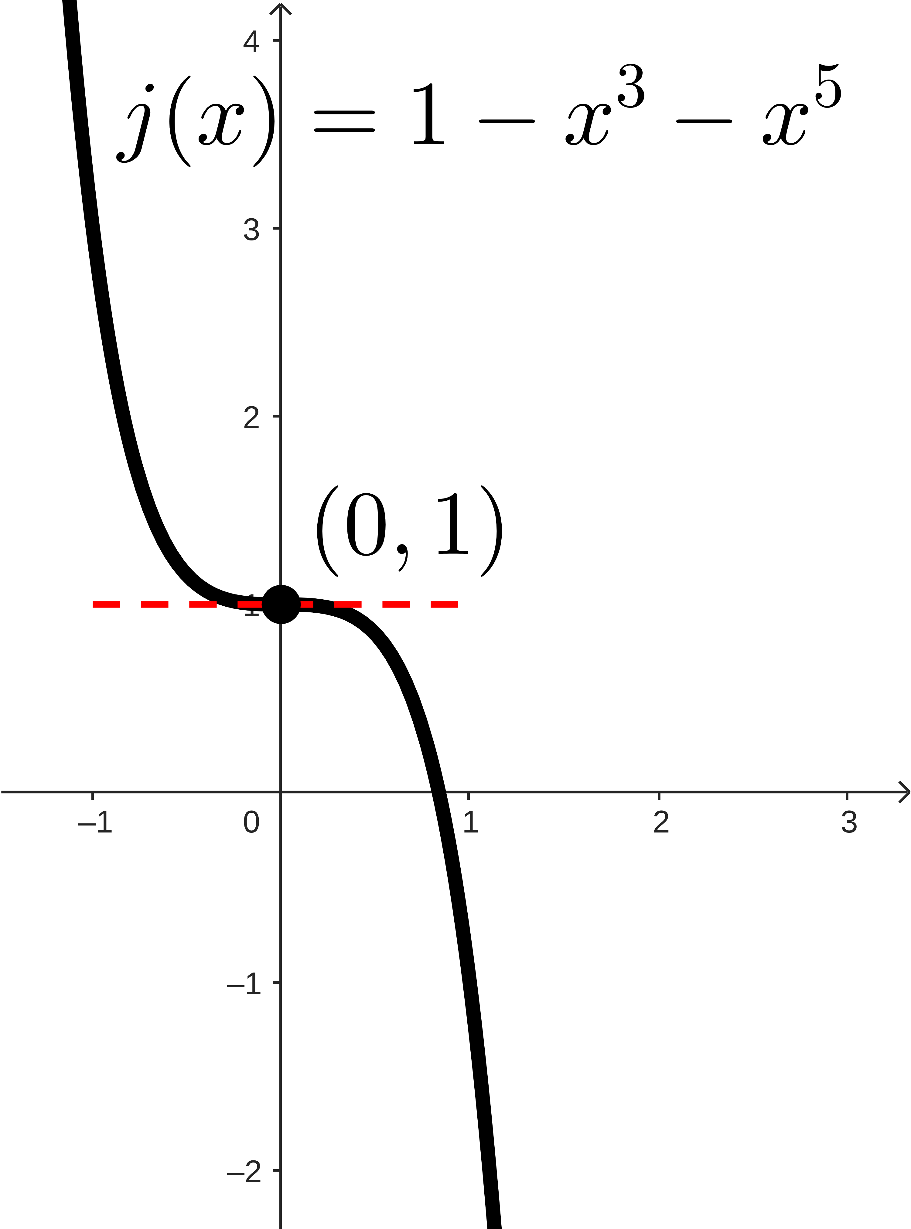
In each graph, find and identify:
  • The intervals where the function is increasing.
  • The intervals where the function is decreasing.
  • The points (or locations) around and between these intervals, the points where the function changes direction or the direction terminates.

(b)

Make a conjecture about the behavior of a function at any point where the function changes direction.
Hint.
What do you think has to be true about the derivative at these points?

(c)

Look at the highest and lowest points on each function. You can even include the points that are highest and lowest just compared to the points around it. Make a conjecture about the behavior of the function at these points.
Hint.
What do you think has to be true about the derivative at these points?
We want to turn this little bit of thinking and exploring into some useful definitions for us. To craft these definitions, we need to start with thinking about what we care about and why we might care about it.

Subsection Critical Points, Local Maximums, and Local Minimums

Let’s start by saying what we’re really looking for is the highest and lowest points on a function. These points are interesting, have useful applications, and are difficult to find in general without calculus. We hopefully noticed, though, that these points always end up showing up at the same kinds of locations! They’re points where the direction of a function changes (or terminates).
We also noticed that there are some common characteristics of those points. They’re points where the derivative was either 0 or didn’t exist. So we’ll start by defining these points, and then we’ll define the idea of “highest” and “lowest” points. Then we’ll put together a result that we hopefully noticed here: that the highest and lowest points show up at these points where the derivative is 0 or doesn’t exist.

Definition 4.2.2. Critical Point of a Function.

We say that a point \((c, f(c))\) on the graph of \(y=f(x)\) is a critical point of the function \(f\) if \(f'(c)=0\) or \(f'(c)\) doesn’t exist.
If \((c, f(c))\) is a critical point of \(f\text{,}\) then we sometimes will call \(x=c\) a critical number and \(y=f(c)\) a critical value.
So these are the points we will look for to find the “highest” and “lowest” points.
Now we need to define this idea so that we can build the result that tells us how to find these highest and lowest points.

Definition 4.2.3. Local Maximum/Minimum.

A point \((c,f(c))\) is a local maximum of \(f(x)\) if there is some open interval of real numbers \((a,b)\) around \(x=c\) (that is, \(a\lt c\lt b\)) and \(f(c)\geq f(x)\) for all \(x\)-values in the intersection of \((a,b)\) and the domain of \(f\text{.}\)
Similarly, a point \((c,f(c))\) is a local minimum of \(f(x)\) if there is some open interval of real numbers \((a,b)\) around \(x=c\) (that is, \(a\lt c\lt b\)) and \(f(c)\leq f(x)\) for all \(x\)-values in the intersection of \((a,b)\) and the domain of \(f\text{.}\)
These are really just slightly technical ways of saying that \(f(c)\) is either the highest or lowest \(y\)-value produced by the function \(f\) for the \(x\)-values near \(x=c\text{.}\)
Now we want to build the connection between these points. In Activity 4.2.1, we pointed out that the highest and lowest points on a function all had the common theme of showing up at places where the derivative was 0 or didn’t exist.
WAIT! STOP! Before you move on, let’s make sure we understand what this theorem is saying. Or maybe what this theorem is not saying.
Notice that we are not saying that every critical point is a local maximum or local minimum! This is a classic “every square is a rectangle but not every rectangle is a square” situation.
Every local maximum/minimum occurs at a critical point, but not every critical point is a local maximum/minimum.

Subsection Direction of a Function (and Where it Changes)

Let’s build up a way of classifying critical points as local maximums, local minimums, or neither.

Activity 4.2.2. Comparing Critical Points.

Let’s think about four different functions:
  • \(\displaystyle f(x) = 4+3x-x^2\)
  • \(\displaystyle g(x) = \sqrt[3]{x+1}+1+x\)
  • \(\displaystyle h(x)=(x-4)^{2/3}\)
  • \(\displaystyle j(x)=1-x^3-x^5\)
Our goal is to find the critical points on the interval \((-\infty,\infty)\) and then to try to figure out if these critical points are local maximums or local minimums or just points that the function increases or decreases through.
(a)
To start, we’re going to be finding critical points. Without looking at a picture of the graph of the function, find the derivative.
Are there any \(x\)-values (in the domain of the function) where the derivative doesn’t exist? We are normally looking for things like division by 0 here, but we could be finding more than that. Check out When Does a Derivative Not Exist? to remind yourself if needed.
Are there any \(x\)-values (in the domain of the function) where the derivative is 0?
(b)
Now that we have the critical points for the function, let’s think about where the derivative might be positive and negative. These will correspond to the direction of a function, based on Theorem 4.1.5 Sign of the Derivative and Direction of a Function.
Write out the intervals of \(x\)-values around and between your list of critical points. For each interval, what is the sign of the derivative? What do these signs mean about the direction of your function?
(c)
Without looking at the graph of your function:
  • What changes about how your function increases up to or decreases down to a critical point based on whether the derivative was 0 or the derivative didn’t exist?
  • Does your function change direction at a critical point? What will that look like, whether it does or does not change direction?
(d)
Give a basic sketch of your graph. It might be helpful to find the \(y\)-values for any critical points you’ve got. Then you can sketch your function increasing/decreasing in the intervals between these points.
In your sketch, include enough detail to tell whether the derivative is 0 or doesn’t exist at each critical point.
(e)
Compare your sketch to the actual graph of the function (you can find all of the graphs in the hint).
Hint.
A graph of f(x). It is a parabola that increases up to a horizontal tangent line a the point (3/2, 25/4), and then decreases away from it.
A graph of g(x). It increases to a vertical tangent line at (-1,0), and then continues increases from there.
A graph of h(x). It decreases down to a vertical tangent line at (4,0), and then increases away from it, forming a cusp or sharp corner.
A graph of j(x). It decreases down to a horizontal tangent line at (0,1), and then decreases away from it.
Figure 4.2.5.
This is great, we have a nice strategy for thinking about critical points!
Something we can notice in finding these critical points (as well as thinking about the domain of the function), we found all of the locations where the derivative is both not positive and not negative. This is a weird way of saying that all of the intervals in between the critical points we found and any breaks in the domain of the function (like if there were vertical asymptotes or holes or something) are places where the derivative is positive or negative.
Even more exciting: if the derivative function we found is continuous, then the Intermediate Value Theorem says that it will only change signs at these critical points (or places like vertical asymptotes or holes). So this means that we can always construct a little chart or something, think about the \(x\)-values around and at critical points or other breaks in the domain, and then look at what the derivative does as we move through those intervals and \(x\)-values.
This will serve as a nice way of thinking about what’s going on with our functions!

Subsection Using the Graph of the First Derivative

Activity 4.2.3. First Derivative Test Graphically.

Let’s focus on looking at a picture of a derivative, \(f'(x)\text{,}\) and trying to collect information about the function \(f(x)\text{.}\) This is what we’ve done already, except that we’ve done it by thinking about the representation of \(f'(x)\) as a function rule written out with algebraic symbols. Here we’ll focus on connecting all of that to the picture of the graphs.
For all of the following questions, refer to the plot below. You can add information with the hints whenever you need to. Don’t reveal the picture of \(f(x)\) until you’re really ready to check what you know.
(a)
Based on the graph of \(f'(x)\text{,}\) estimate the interval(s) of \(x\)-values where \(f(x)\) is increasing.
(b)
Based on the graph of \(f'(x)\text{,}\) estimate the interval(s) of \(x\)-values where \(f(x)\) is decreasing.
(c)
Find the \(x\)-values of the critical points of \(f(x)\text{.}\) Once you’ve estimated these, classify them as local maximums, local minimums, or neither. Explain your reasoning.
(d)
What do you think the graph of \(f(x)\) looks like? Do your best to sketch it or explain it before revealing it!
(e)
Why could we estimate the \(x\)-values of the critical numbers of \(f(x)\text{,}\) but not find the actual coordinates? How come we can’t find the \(y\)-value based on looking at the graph of \(f'(x)\text{?}\)
Reading the graphs of functions is, in general, an important skill. But it’s an especially important idea to be able to read and understand the graph of a function like a derivative and then interpret what we are seeing into some other context.
So for us to really excel here, we’ll want to focus on the fact that a first derivative tells about the slope or direction of a function. Whatever \(y\)-values we find on the graph of a \(f'(x)\) needs to be interpreted as a slope or rate of change of \(f(x)\text{.}\) Then we can string these slopes or rates of changes together to try to think about the behavior of \(f(x)\) by knowing how the \(y\)-values are changing as we move along the curve of \(y=f(x)\text{!}\)

Subsection Strange Domains

We’ll look at two more examples, both of them using functions whose domain is not \((-\infty, \infty)\text{.}\)

Example 4.2.7.

(a)
Consider the function
\begin{equation*} f(x) = \dfrac{x^2}{(x-3)^2}\text{.} \end{equation*}
Find the domain of \(f\text{,}\) the critical points of \(f\text{,}\) and then the intervals where \(f\) is increasing/decreasing. Then, classify any critical points local maximums/minimums if necessary.
Hint 1.
\(f'(x) = -\dfrac{6x}{(x-3)^3}\)
Hint 2.
The function \(f(x)\) has one critical point at \((0,0)\text{.}\) Why isn’t there a critical point at \(x=3\text{?}\) What is happening there instead?
Hint 3.
\(x\)
\((-\infty, 0)\)
\(0\)
\((0,3)\)
\(3\)
\((3,\infty)\)
\(f'\)
\(f\)
Answer.
The domain of \(f(x)\) is \((-\infty, 3)\cup(3,\infty)\) due to the vertical asymptote at \(x=3\text{.}\) The only critical point is at \((0,0)\text{.}\) The table below shows where \(f\) is increasing and decreasing, as well as any local maximums or minimums.
\(x\)
\((-\infty, 0)\)
\(0\)
\((0,3)\)
\(3\)
\((3,\infty)\)
\(f'\)
\(\ominus\)
\(0\)
\(\oplus\)
\(\va\)
\(\ominus\)
\(f\)
\(\searrow\)
\((0,0)\)
\(\nearrow\)
\(\va\)
\(\searrow\)
decreasing
local min
increasing
asymptote
decreasing
(b)
Consider the function
\begin{equation*} g(x) = \sqrt{x}-x+1\text{.} \end{equation*}
Find the domain of \(g\text{,}\) the critical points of \(g\text{,}\) and then the intervals where \(g\) is increasing/decreasing. Then, classify any critical points local maximums/minimums if necessary.
Hint 1.
\(g'(x)=\dfrac{1}{2\sqrt{x}}-1\)
Hint 2.
Notice that, by our definition of critical points, both \((0,1)\) and \(\left(\frac{1}{4},\frac{3}{4}\right)\) are critical points.
Hint 3.
\(x\)
\(0\)
\(\left(0,\frac{1}{4}\right)\)
\(\frac{1}{4}\)
\(\left(\frac{1}{4},\infty\right)\)
\(g'\)
\(g\)
Answer.
The domain of \(g(x)\) is \([0,\infty)\text{.}\) There are two critical points: one at \((0,1)\) and another at \(\left(\frac{1}{4},\frac{3}{4}\right)\text{.}\) The table below shows where \(g\) is increasing and decreasing, as well as any local maximums or minimums.
\(x\)
\(0\)
\(\left(0,\frac{1}{4}\right)\)
\(\frac{1}{4}\)
\(\left(\frac{1}{4},\infty\right)\)
\(g'\)
DNE
\(\ominus\)
\(0\)
\(\oplus\)
\(g\)
\((0,1)\)
\(\searrow\)
\(\left(\frac{1}{4},\frac{3}{4}\right)\)
\(\nearrow\)
local max
decreasing
local min
increasing
So we have two things to notice:
  1. When we have some gap or missing spot in the domain of a function, that can still divide up the intervals where our function is increasing or decreasing! We should notice, though, that since this isn’t actually a point on the curve of our function, it won’t be a critical point and so we have to interpret it differently: we can’t use the First Derivative Test!
  2. An ending point of an interval is a location where the derivative cannot exist! We could define a one-sided derivative (similar to how we defined one-sided continuity in Definition 1.6.2), but for now we’ll just say that the derivative doesn’t exist, and call those ending points critical points. That means that depending on the direction that a function goes away (or leading up to) that ending point, we can classify it as a local maximum or minimum.
Lastly, just a couple of notes: in these little tables or charts (sometimes called sign charts, since they are showing the signs of the derivative), we’ll use some shorthand notation. In Example 4.2.7, we used “DNE” to mean that a derivative “does not exist” at a point. Similarly, we used \(\va\) to represent the vertical asymptote at that \(x\)-value (so that we didn’t accidentally think it was a local maximum or minimum based on the signs of the derivative around it).
Moving forward, we’ll use this same kind of analysis to think about how the derivative might be changing on these intervals. This rate of change of the slopes, the second derivative, will be a useful tool for gathering more information about how a function might be acting.

Practice Problems Practice Problems

1.

Explain what a critical number of \(f(x)\) is. What are the things we’re looking for?

2.

For the following functions, find the critical numbers and explain each one. Is it one where the derivative is 0, or one where the derivative doesn’t exist? Feel free to confirm these by graphing the function!
(a)
\(f(x) = x^2+5x-4\) on \([-4,2]\)
(b)
\(f(x) = \sqrt[3]{x+4}\) on \([-6,-2]\)
(c)
\(f(x) = \dfrac{x^2+1}{x-3}\)
(e)
\(f(x) = x^2 e^{-x}\) on \([1, 10]\)
(f)
\(f(x) = \ln\left(x^{4}+x+1\right)\)

3.

Find the critical numbers of the function \(f(x)\text{,}\) graphed below. Explain each one.
A function that decreases until the point (-2,-1), where it turns around (like a parabola) up to an open hole at (0,1). Then it jumps to a point at (0,2), and increases until it turns around at x=1 (like a parabola). It decreases until x=3. There is a sharp corner as it increases away from the point.
Figure 4.2.8. Graph of \(f(x)\text{.}\)

4.

Give an example of a function that has \(f'(x)\gt 0\) on \((-\infty, 4)\) and \(f'(x)\lt 0\) on \((4,\infty)\text{.}\) Show graphically where the function is increasing and decreasing. Explain how to find out the location of a local maximum or minimum for your example.

5.

Sketch a graph of a function that increases everywhere, but has \(f'(4)=0\text{.}\) Explain what sign the derivative is when \(x\neq 4\text{.}\)

6.

For each of the following functions, use the first derivative to find the intervals where the function is increasing or decreasing.
(e)
\(f(x) = \dfrac{x-4}{x^2+1}\)
(g)
\(f(x) = \dfrac{\sqrt{x}}{e^x}\)
(h)
\(f(x) = \sin(x)\) on \(\left[0, \frac{\sqrt{\pi}}{2}\right]\)
(i)
\(f(x) = \cos^3(x)\) on \((-2\pi, 2\pi)\)

7.

Explain how the First Derivative Test helps us classify critical numbers as local maximums or minimums.

8.

Find any local maximums or local minimums for each of the following functions. Note that these are the same functions that you’ve already worked with in Practice Problem 3.
(e)
\(f(x) = \dfrac{x-4}{x^2+1}\)
(g)
\(f(x) = \dfrac{\sqrt{x}}{e^x}\)
(h)
\(f(x) = \sin(x)\) on \(\left[0, \frac{\sqrt{\pi}}{2}\right]\)
(i)
\(f(x) = \cos^3(x)\) on \((-2\pi, 2\pi)\)

9.

Sketch a graph of a function \(f(x)\) that is continuous on \((-\infty,\infty)\) and has the following characteristics. Label the intervals where \(f\) is increasing/decreasing, and find the locations of any local maximums/minimums.

10.

Sketch a graph of a function \(f(x)\) and has the following characteristics. Label the intervals where \(f\) is increasing/decreasing, and find the locations of any local maximums/minimums.
  • \(f'(x) \lt 0\) on \((-\infty,3)\)
  • \(\displaystyle f'(3) = 0\)
  • \(f'(x)\gt 0\) on \((3,6)\)
  • \(f(x)\) has a vertical asymptote at \(x=6\)
  • \(f'(x)\lt 0\) on \((6,\infty)\)