Let’s remind ourselves of how we interpret derivatives. We are going to repeat a task that we did in Activity 4.2.3 First Derivative Test Graphically. It should feel familiar, which is good! We’re going to use the intuition to make the big connection we’ve been forecasting so far.
Activity5.4.1.Interpreting the Graph of a Derivative.
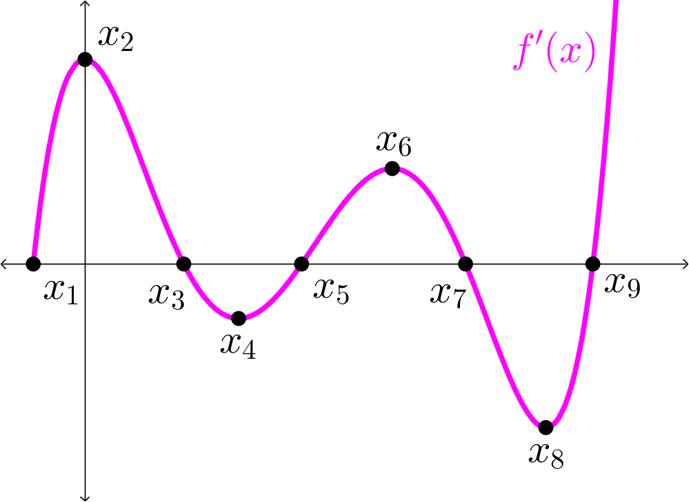
Let’s look at a picture of a graph of the first derivative, \(f'(x)\text{,}\) and try to get some information about \(f(x)\) from it. Use the following graph of \(f'(x)\text{,}\) the first derivative, to answer the questions about \(f(x)\text{.}\)
Since we don’t have a huge amount of detail, you’ll likely have to estimate the \(x\)-values for intervals and points in the following questions, but that’s ok! Estimate away! Just make sure you know what you’re looking for in the graph of \(f'(x)\) to answer these questions.
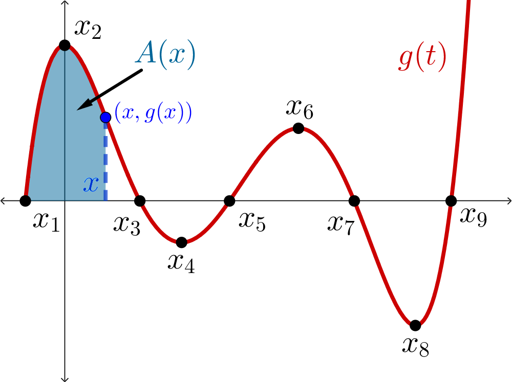
This is a strange function, because we’re defining the function as an integral of another function. Specifically, note that the input for our area function \(A(x)\) is the ending limit of integration: we’re calculating the signed area “under” the curve of \(g(t)\) from \(t=0\) up to some variable ending point \(t=x\text{.}\)
We can visualize this function by looking at the areas we create as we change \(x\text{.}\) For now, get used to just seeing the area “under” \(g\) when we move the point around. The areas themselves are the outputs of the function \(A(x)\text{.}\)
There it is! The way that we can interpret antiderivatives of functions! We found that the derivative of the function that tells us the signed area trapped between a curve and the \(x\)-axis between a fixed starting point and a variable ending point is the curve itself.
Another way of saying this, though, is that the function that tells us the signed area trapped between a curve and the \(x\)-axis between a fixed starting point and a variable ending point is an antiderivative of the curve itself! This is the Fundamental Theorem of Calculus, or at least half of it.
Theorem5.4.1.Fundamental Theorem of Calculus (Part 1).
For a function \(f\) that is continuous on an interval \([a,b]\text{,}\) and a function \(A(x) = \displaystyle\int_{t=a}^{t=x} f(t)\;dt\) defined for \(x\)-values in \([a,b]\text{,}\) then \(A'(x) = f(x)\text{.}\) That is:
The proof of this theorem is one of the most delightful proofs we’ll see. This is a “connector” theorem: a theorem that brings together several big ideas or objects from one common area of math and links them together. Let’s enjoy the proof together.
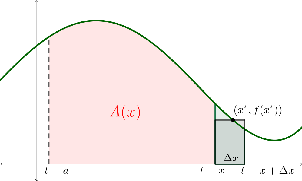
Let \(f(t)\) be a function that is continuous on the interval \(a\leq t\leq b\text{.}\) Then, we’ll define the area function as \(A(x) = \displaystyle \int_{t=a}^{t=x} f(t)\;dt\) for \(a\leq x \leq b\text{.}\) We are interested in \(A'(x)\text{.}\)
The total width of our interval is \(\Delta x\text{,}\) so we have that
\begin{equation*}
\int_{t=x}^{t=x+\Delta x} f(t)\;dt \approx f(x^*) \Delta x
\end{equation*}
where \(x^*\) is some \(x\)-value in \([x, x+\Delta x]\text{.}\) Note that we don’t have a sum, as we normally would, since we are only “adding” a single area of a single rectangle.
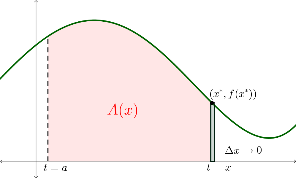
As \(\Delta x\to 0\text{,}\) the options for \(x^*\) in \([x,x+\Delta x]\) reduce to just \(x\text{,}\) since the interval collapses towards the single value. So as \(\Delta x\to 0\text{,}\) we have \(x^*\to x\text{.}\)
To be convinced that \(A'(x)\to f(x^*)\text{,}\) we just have to rely on the fact that, while our Riemann sum only has \(n=1\) rectangle, as \(\Delta x\to 0\) the width(s) of “all” of our rectangles (our only one) approach 0, and so we end up with the definition of a definite integral in the limit:
\begin{align*}
\lim_{\Delta x \to 0} f(x^*)\Delta x \amp = \lim_{\Delta x \to 0} \sum_{k=1}^1 f(x_k^*) \Delta x \\
\amp = \lim_{\Delta x \to 0} \int_{t=x}^{t=x+\Delta x} f(t)\;dt
\end{align*}
Hopefully it is easy to see that \(x^*\to x\text{,}\) since \([x, x+\Delta x]\) collapses on \(x\text{.}\)
This completes the proof! Most of the proofs that you might see for this theorem use the Mean Value Theorem to help, since we can see a connection between the derivative \(A'(x)\) and the average rate of change of the area function:
This theorem is going to be the big result that we use to show how to actually evaluate an area, and so it is easy to think of it as purely support for a “more important” result coming next. But we should pause and think about what this result tells us.
Guaranteeing that every continuous function has an antiderivative family. We have found a function whose derivative is whatever continuous function we want!
Generating antiderivatives. Until now, we have had to rely on being able to recognize functions as derivatives of other things, or be able to “undo” derivative rules. And this will continue to be an important way for us to antidifferentiate functions. But now we have a way of constructing antiderivatives, albeit weird looking ones. We are not yet used to thinking about a function that is defined as a definite integral with a variable ending point.
We will play with this idea more later (in Section 6.1), and so for now we will push forward towards our goal of evaluating a definite integral without directly calculating a limit of Riemann sums.
For \(F(a)\text{,}\) you can evaluate your antiderivative at \(x=a\text{.}\) The important part is thinking about how these two values are different from each other.
For \(F(b)\text{,}\) you can evaluate your antiderivative at \(x=b\text{.}\) The important part is thinking about how these two values are different from each other. Is the difference between these values the same, or different from the difference between \(A(a)\) and \(F(a)\text{?}\)
Phew, this was a lot! Let’s sit back a bit and enjoy the fruits of all of this deep, mathematical thinking: we have a relatively straight-forward way of evaluating definite integrals!
Find an antiderivative of the integrand. (Any antiderivative will do, so we can just choose the one with 0 as the constant term!)
Why is this area 0? What does that mean about the region trapped between \(y=\sin(x)-\cos(x)\) and the \(x\)-axis between \(x=0\) and \(x=2\pi\text{?}\)
This value is \(\frac{14}{3}-e^4+e \approx -47.21\text{.}\) Why is this value negative? What does that mean about the region we’re looking at, and the function we’re looking at?
The Fundamental Theorem of Calculus comes in two parts. Explain why the Fundamental Theorem of Calculus (Part 1) guarantees that any function that is continuous on an interval has an antiderivative on that interval.