Derivatives of Inverse Functions

Section 3.2 Derivatives of Inverse Functions

We should start here by saying: we’re going to be thinking about inverse functions, and so maybe it will be helpful to recap some facts about inverse functions.

If \(y=f(x)\) is some function, then we can use the inverse function to represent this relationship between variables: \(x=f^{-1}(y)\text{.}\) Some examples:
- \(y=e^x \longleftrightarrow x=\ln(y)\text{.}\) That is, the logarithm function “solves” for the exponent (sometimes this is easier to just say that the logarithm is the exponent).
  🔗
  
  🔗
- \(y=\sin(\theta)\longleftrightarrow \theta =\sin^{-1}(y)\text{.}\) That is, this inverse sine function (or sometimes \(\arcsin(y)\)) finds the angle at which sine of that angle is \(y\text{.}\) With these trigonometric functions, we need to make some restrictions: because there are an infinite number of angles that will produce the same output of the sine function (reflecting the angle across the \(y\)-axis will do it, as will adding any multiple of \(2\pi\)), we restrict the angles that the inverse sine function can output to being in \(\left[-\frac{\pi}{2}, \frac{\pi}{2}\right]\text{.}\)
  🔗
  
  🔗
🔗
🔗
Based on this re-representation above, we can always compose a function and its inverse to get the identity function, \(y=x\text{.}\) In general, if \(y=f(x)\) has an inverse function \(f^{-1}\text{,}\) then \(\left(f\circ f^{-1}\right)(x)=f\left(f^{-1}(x)\right) = x\text{.}\) Similarly, we can compose in the opposite order: \(\left(f^{-1}\circ f\right)(x) = f^{-1}\left(f(x)\right) = x\text{.}\) This can be a bit trickier to think about for the inverse trigonometric functions, since this only works on intervals of \(x\) where that inverse is defined. So we end up with strange things like:

\begin{equation*} \sin^{-1}\left(\sin\left(\frac{3\pi}{2}\right)\right) = \sin^{-1}\left(-1\right) = -\frac{\pi}{2}\text{.} \end{equation*}

This is because the inverse sine function finds only angles in the interval \(\left[-\frac{\pi}{2}, \frac{\pi}{2}\right]\text{,}\) and the angles \(\frac{3\pi}{2}\) and \(-\frac{\pi}{2}\) are coterminal (and so have the same output from the sine function).

🔗

🔗

With these small facts in mind, we can think about derivatives of inverse functions.

🔗

Subsection Wielding Implicit Differentiation

We’re going to do a very cool thing: in order to find derivatives of inverse functions, we can invert the relationship between \(x\) and \(y\text{,}\) and then use Implicit Differentiation to find \(\dydx\text{.}\)

🔗

Activity 3.2.1. Building the Derivative of the Logarithm.

We’re going to accomplish two things here:

By the end of this activity, we’ll have a nice way of thinking about \(\ddx{\ln(x)}\text{,}\) and we will now be able to differentiate functions involving logarithms!
🔗

🔗
Throughout this activity, we’re going to develop a way of approaching derivatives of inverse functions more generally. Then we can apply this framework to other functions!
🔗

🔗

Let’s think about this logarithmic function!

🔗

(a)

We have stated (a couple of times now) how we define the log function:

\begin{equation*} y=e^x \longleftrightarrow x=\ln(y)\text{.} \end{equation*}

This arrow goes both directions: the log function is the inverse of the exponential, but the exponential is the inverse of the log function!

🔗

Can you rewrite the relationship \(y=\ln(x)\) using its inverse (the exponential)?

🔗

(b)

For your inverted \(y=\ln(x)\) from above (it should be \(x=\fillinmath{XXXXX}\)), apply a derivative operator to both sides, and use implicit differentiation to find \(\dydx\) or \(y'\text{.}\)

🔗

Hint.

Where do we have to use the Chain Rule?

🔗

(c)

A weird thing that we can notice is that when we use implicit differentiation, it is common to end up with our derivative written in terms of both \(x\) and \(y\) variables. This makes sense for our earlier examples: we needed specific coordinates of the point on the circle, for instance, to find the slope there.

🔗

But if \(y=\ln(x)\text{,}\) we want \(\dydx\) or \(y'\) to be a function of \(x\text{:}\)

\begin{equation*} f(x)=\ln(x) \longrightarrow f'(x)=\fillinmath{XXXXX}\text{.} \end{equation*}

Your derivative is written with only \(y\) values.

🔗

Since \(y=\ln(x)\text{,}\) replace any instance of \(y\) with the log function. What do you have left?

🔗

(d)

Remember that \(y=\ln(x)\text{.}\) Substitute this into your equation for \(\dydx\text{.}\) Can you write this in a pretty simplistic way?

🔗

Hint.

Remember that \(e^{\ln(x)}=x\text{,}\) since these functions are inverses of each other!

🔗

(e)

Before we go much further, we should be a bit careful. What is the domain of this derivative?

🔗

What are the values of \(x\) where \(\ddx{\ln(x)}\) makes sense to think about?

🔗

Theorem 3.2.1. Derivative of the Logarithmic Function.

\begin{equation*} \ddx{\ln(x)}=\frac{1}{x} \end{equation*}

for \(x\gt 0\text{.}\)

🔗

Further, since \(\log_b(x) = \frac{\ln(x)}{\ln(b)}\) (for \(b\geq 0\) and \(b\neq 1\)), we can say that:

\begin{equation*} \ddx{\log_b(x)} = \frac{1}{x\ln(b)} \end{equation*}

for \(x\gt 0\text{.}\)

🔗

Subsection Derivatives of the Inverse Trigonometric Functions

Let’s try a similar thing with inverse trigonometric functions. We’ll start with the inverse sine function, \(y=\sin^{-1}(x)\text{.}\)

🔗

Activity 3.2.2. Finding the Derivative of the Inverse Sine Function.

We’re going to do the same trick, except that there will be a couple of small differences due to thinking specifically about trigonometric functions.

🔗

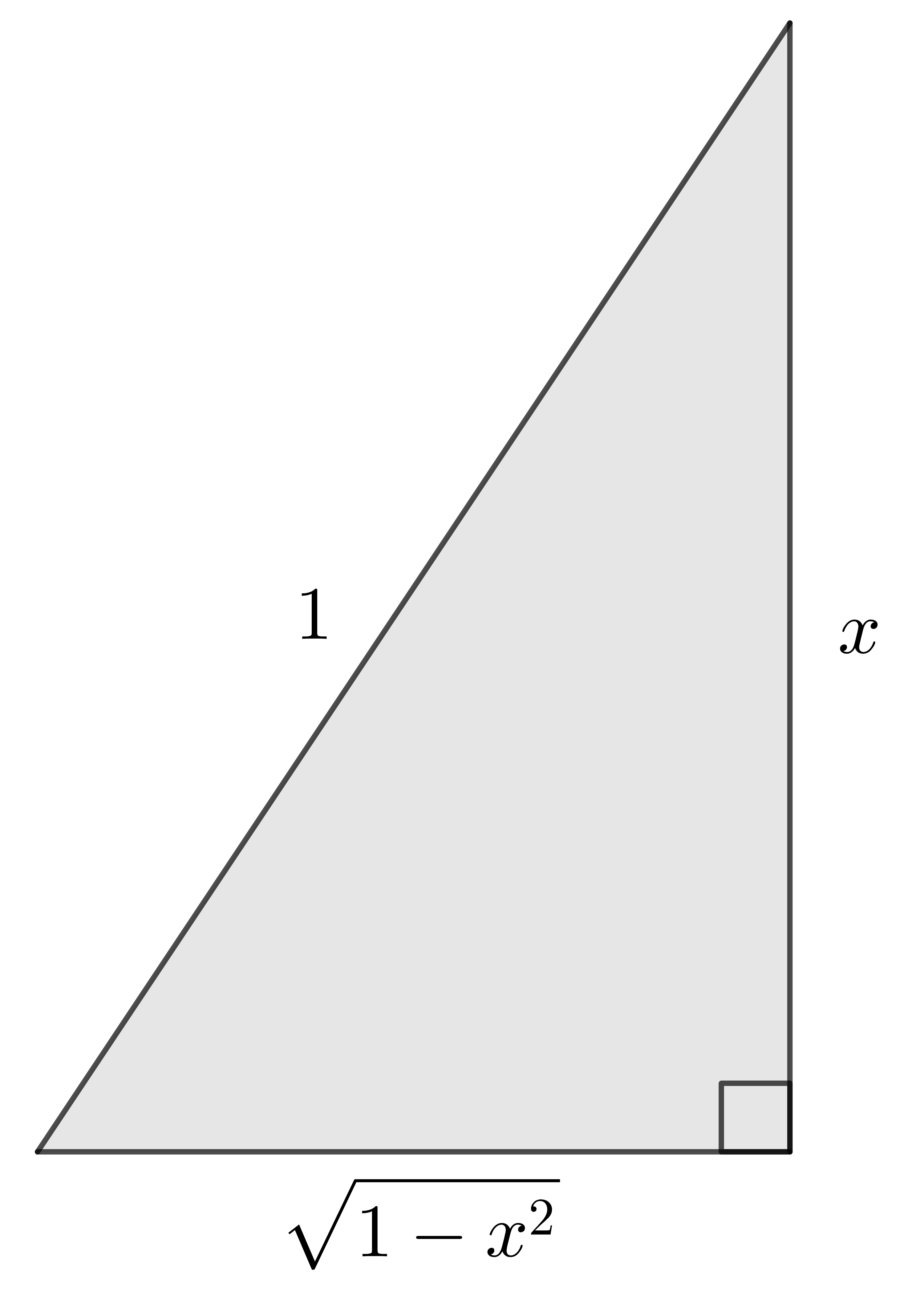
Let’s think about the function \(y=\sin^{-1}(x)\text{.}\) We know that this is equivalent to \(x=\sin(y)\) (for \(y\)-values in \(\left[-\frac{\pi}{2},\frac{\pi}{2}\right]\)).

🔗

(a)

Move the point around the portion of the unit circle in the graph below. Convince yourself that:

\(\displaystyle \sin(y)=x\)
🔗

🔗
\(\sin(y)\geq 0\) when \(0\leq y \leq \frac{\pi}{2}\)
🔗

🔗
\(\sin(y)\lt 0\) when \(-\frac{\pi}{2}\leq y \lt 0\)
🔗

🔗

🔗

What is \(\cos(y)\) in this figure? Does the sign change depending on the value of \(y\text{?}\)

🔗

(b)

Use implicit differentiation and the equation \(x=\sin(y)\) to find \(\dydx\) or \(y'\)

🔗

(c)

If you still have your derivative written in terms of \(y\text{,}\) make sure to write \(\cos(y)\) in terms of \(x\text{!}\)

🔗

(d)

Let’s think about the domain of this derivative: what \(x\)-values make sense to think about?

🔗

Think about this both in terms of what \(x\)-values reasonably fit into your formula of \(\ddx{\sin^{-1}(x)}\) as well as the domain of the inverse sine function in general.

🔗

(e)

Notice that in the denominator of \(\ddx{\sin^{-1}(x)}\text{,}\) you have a square root. Based on that information (and the visual above), what do you expect to be true about the sign of the derivative of the inverse sine function?

🔗

Confirm this by playing with the graph of \(y=\sin^{-1}(x)\) below.

🔗

(f)

Investigate the behavior of \(\dydx\) at the end-points of the function: at \(x=-1\) and \(x=1\text{.}\) What do the slopes look like they’re doing, graphically?

🔗

How does this work when you look at the function you built above? What happens when you try to find \(\Dydx\bigg|_{x=-1}\) or \(\Dydx\bigg|_{x=1}\text{?}\)

🔗

Let’s repeat the process to find the derivatives of \(y=\tan^{-1}(x)\) and \(y=\sec^{-1}(x)\text{.}\)

🔗

Activity 3.2.3. Building the Derivatives for Inverse Tangent and Secant.

(a)

Consider the triangle representing the case when \(y=\tan^{-1}(x)\text{.}\)

🔗

Right triangle with hypotenuse sqrt(x^2+1) and the other side lengths 1 and x. The angle between 1 and sqrt(x^2+1) is labeled y. — Figure 3.2.2.
🔗

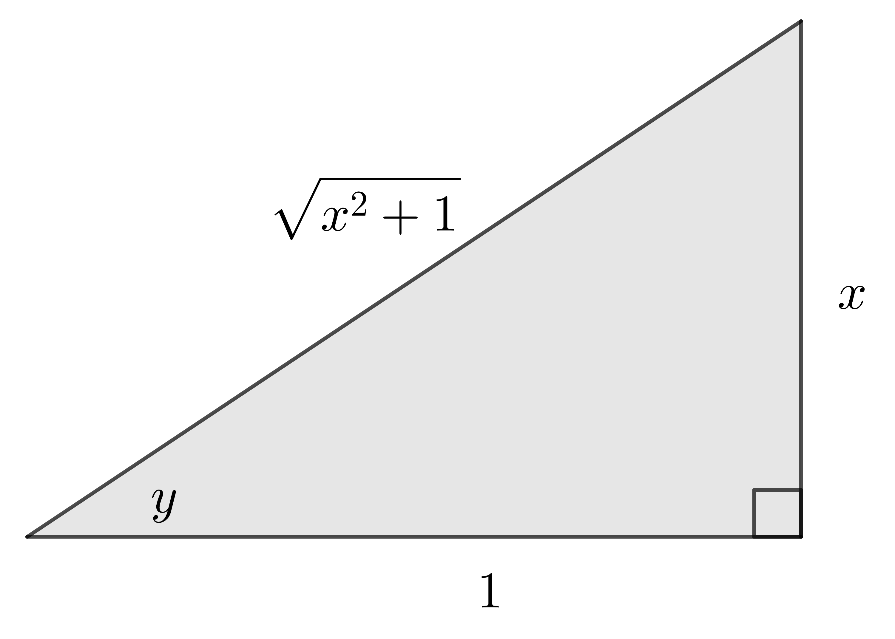
For \(x=\tan(y)\text{,}\) find \(\dydx\) using implicit differentiation. Find an appropriate expression for \(\sec(y)\) based on the triangle above, but we will refer back to the version with the \(\sec(y)\) in it later.

🔗

(b)

Consider the triangle representing the case when \(y=\sec^{-1}(x)\text{.}\)

🔗

Right triangle with hypotenuse x and the other side lengths 1 and sqrt(x^2-1). The angle between 1 and x is labeled y. — Figure 3.2.3.
🔗

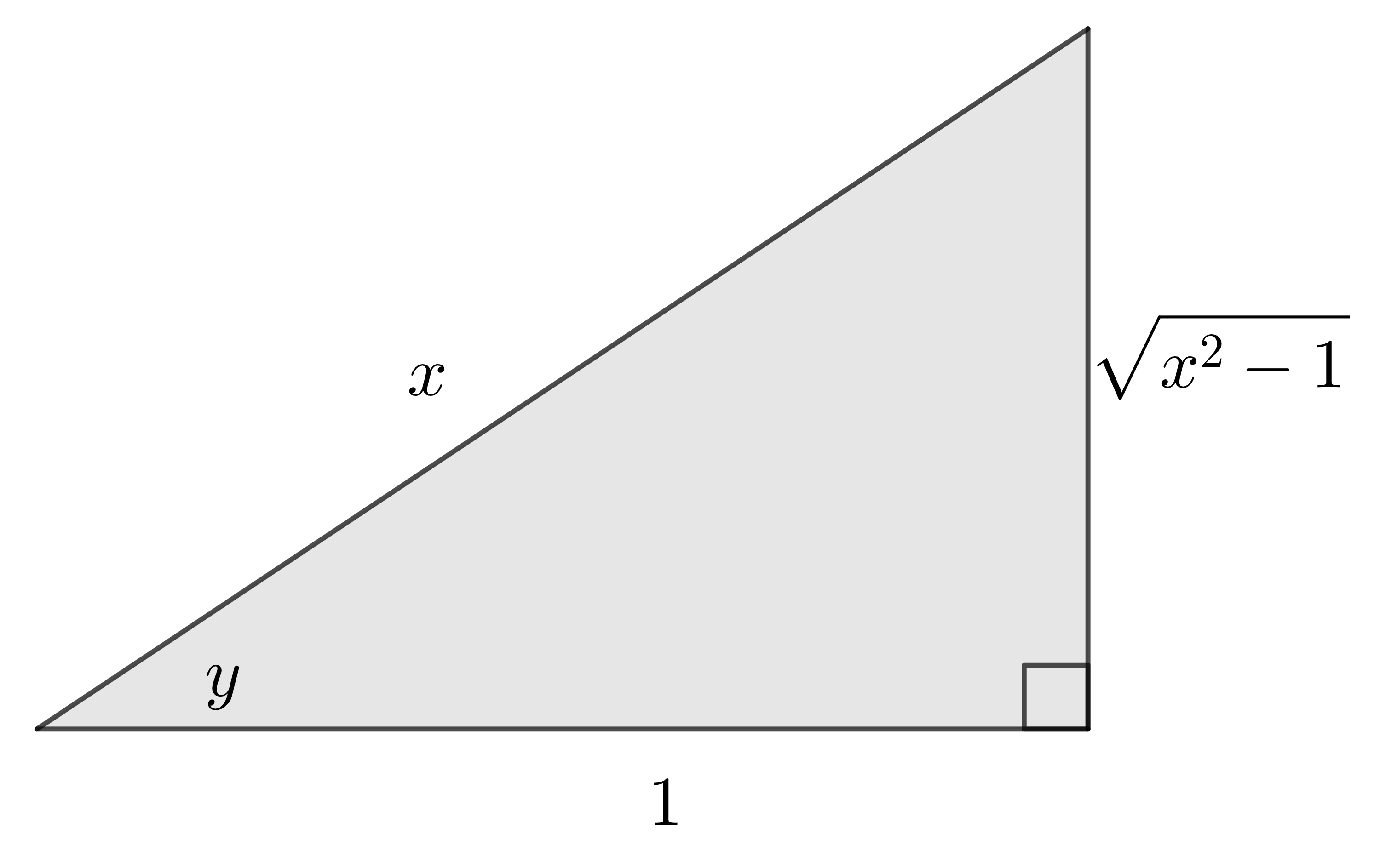
For \(x=\sec(y)\text{,}\) find \(\dydx\) using implicit differentiation. Find an appropriate expression for \(\sec(y)\) and \(\tan(y)\) based on the triangle above, but we will refer back to the version with the functions of \(y\) in it later.

🔗

(c)

Here’s a graph of just the unit circle for angles \([0,\pi]\text{.}\) We are choosing to focus on this region, since these are the angles that the inverse tangent and inverse secant functions will return to us. We want to investigate the signs of \(\tan(y)\) and \(\sec(y)\text{.}\)

🔗

(d)

Go back to our derivative expressions for both the inverse tangent and inverse secant functions. What do we know about the signs of these derivatives?

🔗

Hint.

Notice that in \(\ddx{\tan^{-1}(x)} = \frac{1}{\sec^2(y)}\text{,}\) we know that the derivative must be positive. Even when \(\sec(y)\lt 0\text{,}\) we are squaring it.

🔗

In \(\ddx{\sec^{-1}(x)} = \frac{1}{\sec(y)\tan(y)}\text{,}\) we know that the derivative must also always be positive. Whenever \(\sec(y)\lt 0\text{,}\) we have \(\tan(y)\lt 0\text{,}\) and so the product must be positive.

🔗

(e)

Confirm your idea about the sign of the derivatives by investigating the graphs of each function.

🔗

(f)

How do we need to write these derivatives, when we write them in terms of \(x\) to account for the sign of the derivative?

🔗

Hint.

Use an absolute value in the formula for \(\ddx{\sec^{-1}(x)}\text{!}\)

🔗

It is important to think carefully about how things might change when we start thinking about other trigonometric functions. For instance, what happens when we think about \(y=\cos^{-1}(x)\) instead? We could repeat the process from Activity 3.2.2 with \(y=\cos^{-1}(x)\) instead (and we’ll do that for \(y=\tan^{-1}(x)\)), but for now let’s think about the graph of \(y=\cos^{-1}(x)\text{.}\)

🔗

Activity 3.2.4. Connecting These Inverse Functions.

We’re going to look at a graph of \(y=\cos^{-1}(x)\text{,}\) but we’re specifically going to try to compare it to the graph of \(y=\sin^{-1}(x)\text{.}\) We’ll use some graphical transformations to make these functions match up, and then later we’ll think about derivatives.

🔗

(a)

Ok, consider the graph of \(y=\cos^{-1}(x)\) and a transformed version of the inverse sine function. Apply some graphical transformations to make these match!

🔗

(b)

It might be fun to think about another reason that this connection between \(\sin^{-1}(x)\) and \(\cos^{-1}(x)\) exists.

🔗

Consider this triangle:

A right triangle with side lengths labeled x and sqrt(1-x^2) with the hypotenuse labeled 1. — Figure 3.2.4.
🔗

We’re going to think about these inverse trigonometric functions as angles: let \(\alpha = \cos^{-1}(x)\) and \(\beta = \sin^{-1}(x)\text{.}\) We can rewrite these as:

\begin{align*} \cos(\alpha) \amp = x\\ \sin(\beta) \amp =x \text{.} \end{align*}

Can you fill in your triangle using this information?

🔗

Why does \(\alpha + \beta = \frac{\pi}{2}\text{?}\) Convince yourself that this is what we did with the graphical transformations above, as well.

🔗

(c)

Use this equation above, rewriting \(\cos^{-1}(x)\) as some expression involving the inverse sine function, and then find

\begin{equation*} \ddx{\cos^{-1}(x)}\text{.} \end{equation*}

🔗

Hint.

\begin{equation*} \ddx{\cos^{-1}(x)} = \ddx{-\sin^{-1}(x)+\frac{\pi}{2}} \end{equation*}

🔗

We could repeat this task to try to connect the graph of \(y=\tan^{-1}(x)\) with \(y=\cot^{-1}(x)\) as well as the graph of \(y=\sec^{-1}(x)\) with \(y=\csc^{-1}(x)\text{,}\) but we can hopefully see what will happen. In each case, we have the same kind of connection that we saw in the triangle, since these are cofunctions of each other!

🔗

We can summarize by believing that:

\begin{align*} \ddx{\cos^{-1}(x)} \amp =-\ddx{\sin^{-1}(x)} = -\frac{1}{\sqrt{1-x^2}}\\ \ddx{\cot^{-1}(x)} \amp =-\ddx{\tan^{-1}(x)} =-\frac{1}{x^2+1}\\ \ddx{\csc^{-1}(x)} \amp = -\ddx{\sec^{-1}(x)}= -\frac{1}{|x|\sqrt{x^2-1}} \end{align*}

🔗

Theorem 3.2.5. Derivatives of the Inverse Trigonometric Functions.

\begin{align*} \ddx{\sin^{-1}(x)} \amp = \frac{1}{\sqrt{1-x^2}} \amp \text{Domain: }-1\lt x\lt 1\\ \ddx{\cos^{-1}(x)} \amp = -\frac{1}{\sqrt{1-x^2}} \amp \text{Domain: }-1\lt x\lt 1\\ \ddx{\tan^{-1}(x)} \amp = \frac{1}{x^2+1} \amp \text{Domain: all Real numbers} \\ \ddx{\cot^{-1}(x)} \amp = -\frac{1}{x^2+1} \amp \text{Domain: all Real numbers}\\ \ddx{\sec^{-1}(x)} \amp = \frac{1}{|x|\sqrt{x^2-1}} \amp \text{Domain: } x\lt -1 \text{ and } x \gt 1\\ \ddx{\csc^{-1}(x)} \amp = -\frac{1}{|x|\sqrt{x^2-1}} \amp \text{Domain: }x\lt -1 \text{ and } x \gt 1 \end{align*}

🔗

Now that we have these new derivative rules for these functions, we can practice applying them! We can use these along with the Product, Quotient, and Chain Rules to differentiate many different functions.

🔗