For the limits and function values above, which of these are you most confident in? What about the limit, function value, or graph of the function makes you confident about your answer?
Similarly, which of these are you the least confident in? What about the limit, function value, or graph of the function makes you not have confidence in your answer?
We’re going to repeat this process, but with a slight change to the representation of each function. Hopefully this will be illuminating in our attempt to add more precision to our estimations.
Activity1.2.2.From Estimating to Evaluating Limits (Part 2).
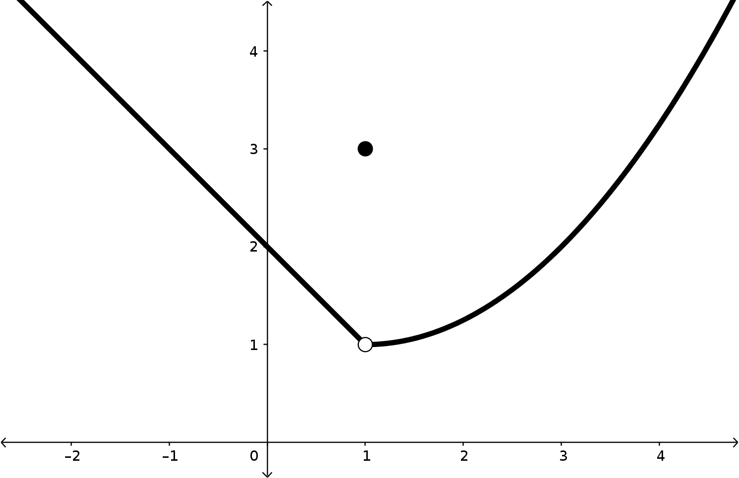
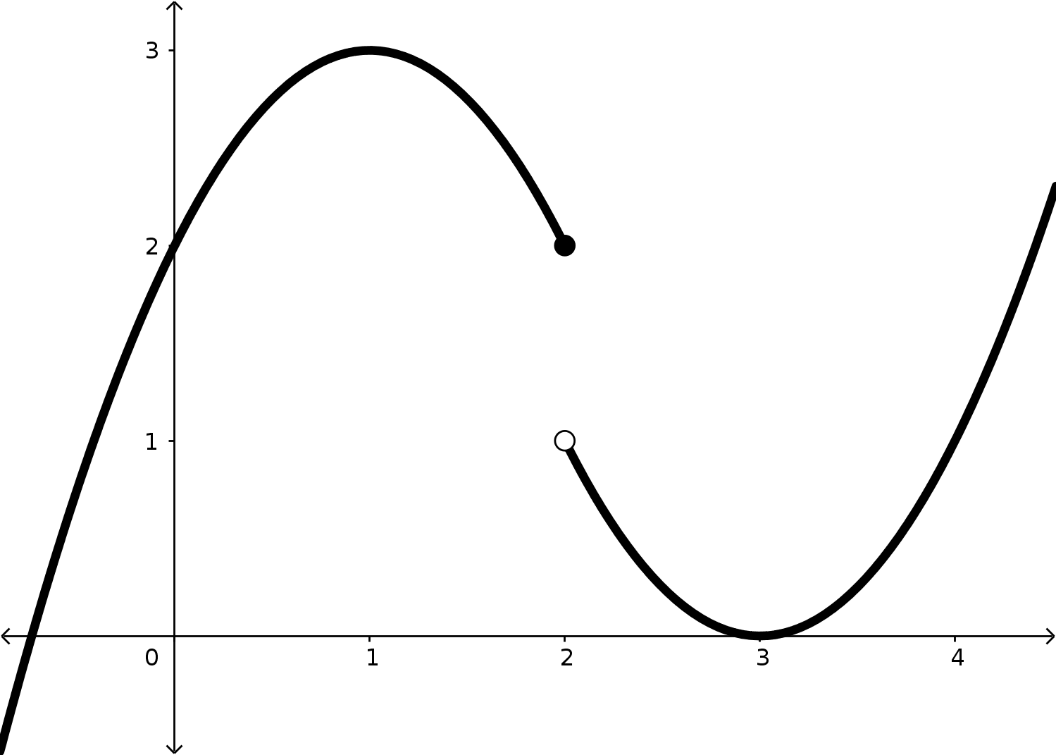
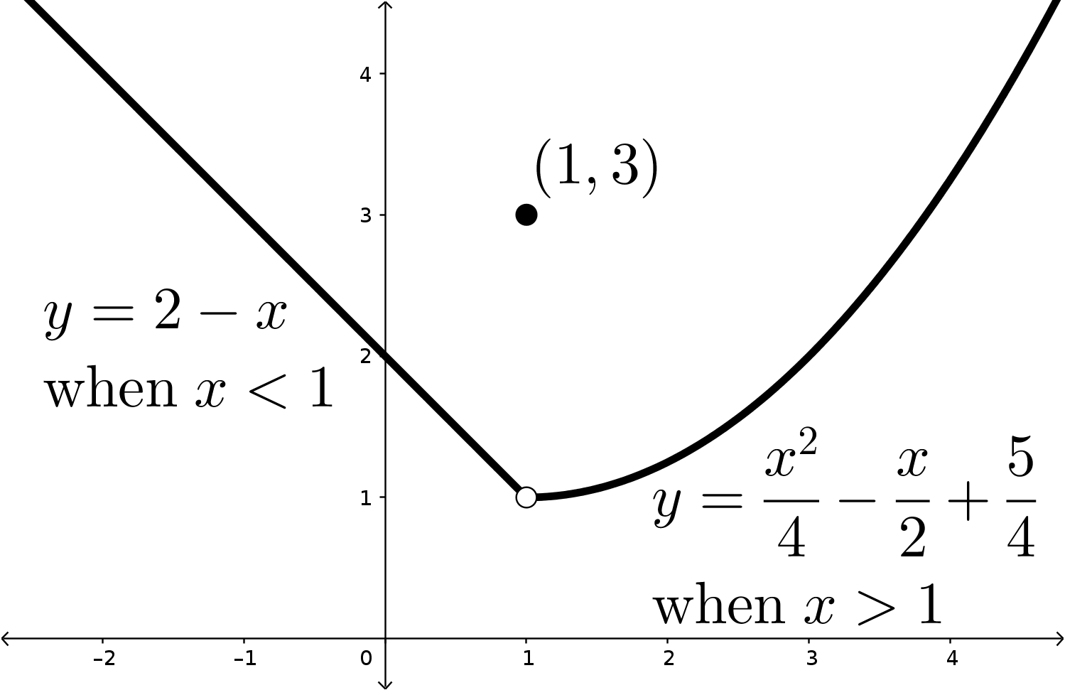
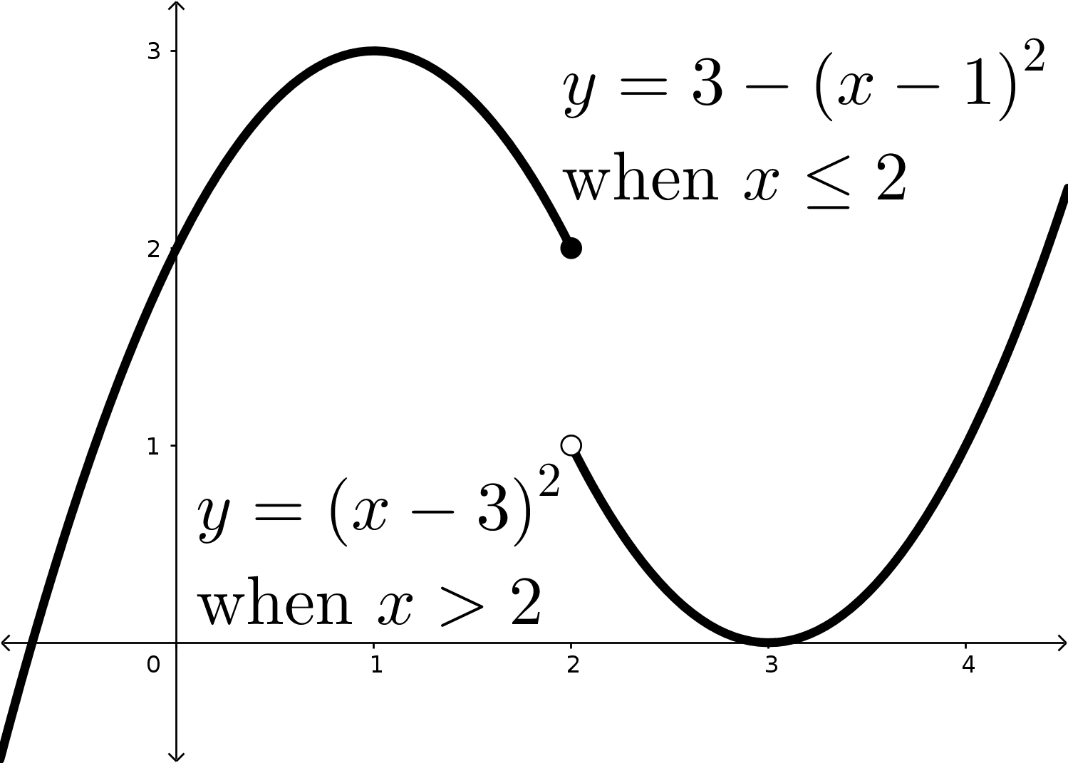
Let’s consider the following graphs of functions \(f(x)\) and \(g(x)\text{,}\) now with the added labels of the equations defining each part of these functions.
Figure1.2.3.Graph of the function \(f(x)\text{.}\)
Does the addition of the function rules change the level of confidence you have in these answers? What limits are you more confident in with this added information?
Find the limits \(\displaystyle \lim_{x\to 1}f(x)\) and \(\displaystyle \lim_{x\to 2}g(x)\text{.}\) Compare these values of \(f(1)\) and \(g(2)\text{:}\) are they related at all?
These two examples are hopefully helpful for us to see that when we are given the actual rule for a function \(f\) that connects \(x\) to the corresponding output \(f(x)\text{,}\) we are able to move past estimation. We suddenly have whatever level of precision we’d like, since we can immediately see what is happening with every \(x\) input to produce the corresponding \(f(x)\) output.
We want to remind ourselves how we can combine functions using different operations, and how we might find outputs based on the different combinations. Our goal is to then think about how this might work with limits: how can we summarize the behavior of combinations of functions around some point?
Let’s consider some functions \(f(x)=x^2+3\) and \(g(x)=x-\dfrac{1}{x}\text{.}\) We’ll say that the domain of both functions is \((0,\infty)\) for our own convenience.
You might think about writing out a function rule for \(h(x)\text{.}\) But can you also find \(h(2)\) without ever writing out a rule for \(h(x)\text{?}\)
If we instead define the function \(h(x)=f(x)-g(x)\text{,}\) how would you describe at least two different ways of finding the value of \(h(2)\text{?}\)
What about a scaled version of one of these functions? If we let \(h(x)=4f(x)\) and \(j(x)=\dfrac{g(x)}{3}\text{,}\) can you describe more than one way to find the value of \(h(3)\) and \(j(3)\text{?}\)
You can probably guess where we’re going: we’re going to define a function that is the product of \(f\) and \(g\text{:}\)\(h(x)=f(x)\cdot g(x)\text{.}\) Describe more than one way of evaluating \(h(4)\text{.}\)
If \(h(x)=\dfrac{f(x)}{g(x)}\text{,}\) then are there any \(x\)-values that are in the domain of \(f\) and \(g\) (the domain is \(x\gt 0\)) that \(h(x)\) cannot be defined for? Why?
Ok, we can confront this big idea: when we combine functions, we can either evaluate the combination of the functions at some \(x\)-value or evaluate each function separately and just combine the answers! Of course, there are some limitations (like when the combination isn’t nicely defined because of division by 0 or something else), but this is a good framework to move forward with!
Maybe this activity was obvious for you, but it might not have been! This isn’t something that we always think about with functions, even if (deep down) we know it to be true.
A nice extension that we can make is that moving past functions evaluated at a specific \(x\)-value towards descriptions of the behavior of functions around that specific \(x\)-value.
We’ll apply this same kind of thinking (combining things by looking at each piece individually first, and then combining the answers together) to limits of combinations of functions.
If \(f(x)\) and \(g(x)\) are two functions defined at \(x\)-values around, but maybe not at, \(x=a\) and \(\displaystyle \lim_{x\to a}f(x)\) and \(\displaystyle \lim_{x\to a}g(x)\) both exist, then we can evaluate limits of combinations of these functions.
Sums: The limit of the sum of \(f(x)\) and \(g(x)\) is the sum of the limits of \(f(x)\) and \(g(x)\text{:}\)
Quotients: The limit of a quotient of \(f(x)\) and \(g(x)\) is the quotient of the limits of \(f(x)\) and \(g(x)\) (provided that you do not divide by 0):
We can summarize these properties: when we are thinking about our basic operations on functions, we can evaluate limits by just looking at the limits of each component function individually and then piecing those individual limit values back together.
This kind of structural “building-block” behavior is a really important one in mathematics. Whenever we define some new mathematical object, properties like this are typically good ideas for us to check in order to learn more about the object we’ve defined.
Ok, let’s move on. We’re going to turn our attention to something more concrete. We’re going to think of two function types: constant functions and the identity function.
These two functions might seem pretty simplistic (most functions that we think of are more complicated than these), but we can use these to build more functions!
We’re going to use a combination of properties from Theorem 1.2.5 and Theorem 1.2.6 to think a bit more deeply about polynomial functions. Let’s consider a polynomial function:
We’re going to evaluate the limit \(\displaystyle \lim_{x\to 1} f(x)\text{.}\) First, use the properties from Theorem 1.2.5 to rewrite this limit as 4 different limits added or subtracted together.
Now, for each of these limits, rewrite them as products of things until you have only limits of constants and identity functions, as in Theorem 1.2.6. Evaluate your limits.
Based on the definition of a limit (Definition 1.1.1), we normally say that \(\displaystyle \lim_{x\to 1} f(x)\) is not dependent on the value of \(f(1)\text{.}\) Why do we say this?
Come up with a new polynomial function: some combination of coefficients with \(x\)’s raised to natural number exponents. Call your new polynomial function \(g(x)\text{.}\) Evaluate \(\displaystyle \lim_{x\to -1} g(x)\) and compare the value to \(g(-1)\text{.}\) Explain why these values are the same.
This leads us to an important result about a whole class of functions: polynomials! We can (finally) evaluate the limit of a polynomial without having to think too carefully about the distinction between the behavior of the function around\(x=a\) and the behavior of the function at\(x=a\text{.}\)
This result really just says that polynomials are friendly functions for limits: sure, a limit is really about the behavior of the function outputs around (but not at) \(x=a\text{,}\) but for polynomial functions, specifically, we can wave our hands and say “Ah, who cares, it’s all the same anyways!”
Are there some typical functions that we’ll work with where this result doesn’t work (and we actually have to be aware of the behavior around a point instead of at it)?
The answers to these questions will come slowly but surely, and we’ll hopefully be able to start using these limits as a tool to think about more interesting and important topics soon: we just need to make sure we’re familiar with them first.
Given \(\displaystyle\lim_{x\to3} f(x) = 5\) and \(\displaystyle \lim_{x\to 3} g(x) = -2\text{,}\) evaluate the following limits. If the limit doesn’t exist, explain why. Write out a few steps and explanations to justify your work.