The Integral Test

Section 8.4 The Integral Test

Subsection Infinite Series As a Kind of Integral

Let’s start here with a connection between objects. We’ve already thought about the connection between an infinite series and the sequence of terms of the series (Theorem 8.3.3 Divergence Test). Now we’ll think about the connections between two objects that are similar to each other in that they both represent an accumulation of function values.

🔗

Earlier (in Sequences as Functions) we tried to describe sequences as just a special kind of function: the domain is the set of non-negative integer (or positive integers, depending on whether we start our index at $n=0$ or $n=1$) and we map these inputs to real number outputs. And now we want to think about what it might mean to accumulate the values of these kinds of functions.

🔗

Function value accumulation is what we’ve been looking at lately! That’s what integration is! We are trying to accumulate all of the function values and weigh them based on their “width.” In the context of continuous functions, that means we start approximating this accumulation by looking at some finite number of function values that we pick, and we give them some $\Delta x$ width between them. That’s our Riemann sum:

\begin{equation*} \sum_{k=1}^n f(x_k^*) \; \Delta x \end{equation*}

And from there, we work on making that space between function values get smaller (as the number of function values we use gets higher). So when $n$ is the number of function values, we can let $n\to \infty$ and correspondingly we get $\Delta x \to dx\text{,}$ the differential in our integral:

\begin{equation*} \lim_{n\to\infty} \sum_{k=1}^n f(x_k^*) \;\Delta x = \int_{x=a}^{x=b}f(x)\;dx\text{.} \end{equation*}

🔗

And this is how we’ve talked about infinite series so far, even adopting the same notions of convergence and thinking about how we extend a familiar idea (in this case adding numbers, compared to integrating a function) out to infinity: we just keep walking our (finite) ending point out to infinity using a limit!

🔗

So this brings us to this comparison of the same types of objects across these two different contexts.

🔗

Table 8.4.1. Comparisons of Calculus Objects in Continuous and Discrete Contexts

🔗

Object	Continuous Context	Discrete Context
Function	$f(x)$	$a_k$
Graph	Figure 8.1.4	Figure 8.1.5
Finite Accumulation	Definite Integral	Partial Sum
	$\displaystyle A(t) = \int_{x=0}^{x=t} f(x)\;dx$	$\displaystyle S_n = \sum_{k=0}^n a_k$
Infinite Accumulation	Improper Integral	Infinite Series
	$\displaystyle\int_{x=0}^\infty f(x)\;dx$	$\displaystyle\sum_{k=0}^\infty a_k$

So in this section, we’ll investigate this link between infinite series and improper integrals as the same kind of object occurring in different contexts. Intuitively, then, they’ll be related to each other, under the right conditions.

🔗

Subsection The Integral Test

The Integral Test is really about connecting the behavior of an integral and a series, and the way that we’ll do it is by trying to visualize what an infinite series is (a sum of function values, where the function inputs are spaced apart by 1) and linking that to a Riemann sum. From there, we’ll use the Monotone Convergence Theorem on the sequence of partial sums to show that the series converges.

🔗

Activity 8.4.1. Integrals and Infinite Series.

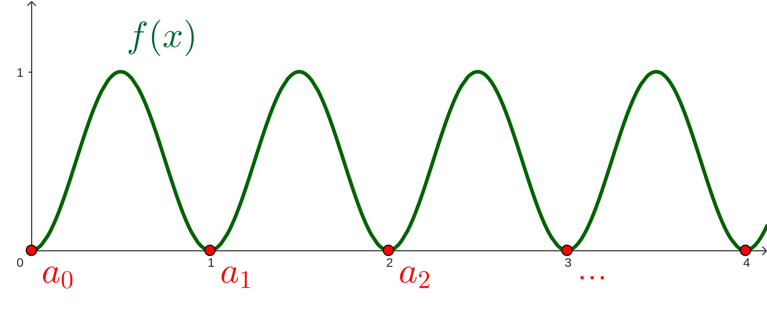
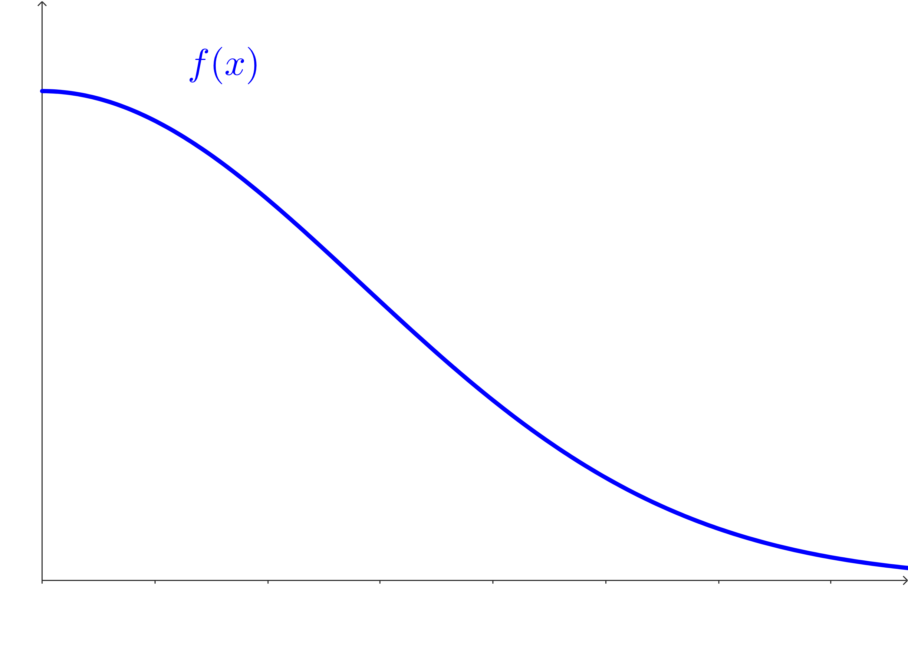
We’re going to work with a graph of a continuous function, and we’re going to start with a couple of conditions:

Our function will be continuous wherever it’s defined.
🔗

🔗
Our function will be decreasing on its domain.
🔗

🔗
All of the function outputs will be positive.
🔗

🔗

Let’s not worry about picking a specific function for this, but we will visualize a graph of one that meets these three requirements.

🔗

A blue curve labeled f(x). The curve is positive, decreasing, and continuous. It is defined on [0,infinity) with, seemingly, a horizontal asymptote at the x-axis. — Figure 8.4.2.
🔗

We can then visualize the sequence of terms, $a_k = f(k)$ for $k=0, 1, 2, ...,\text{.}$

🔗

(a)

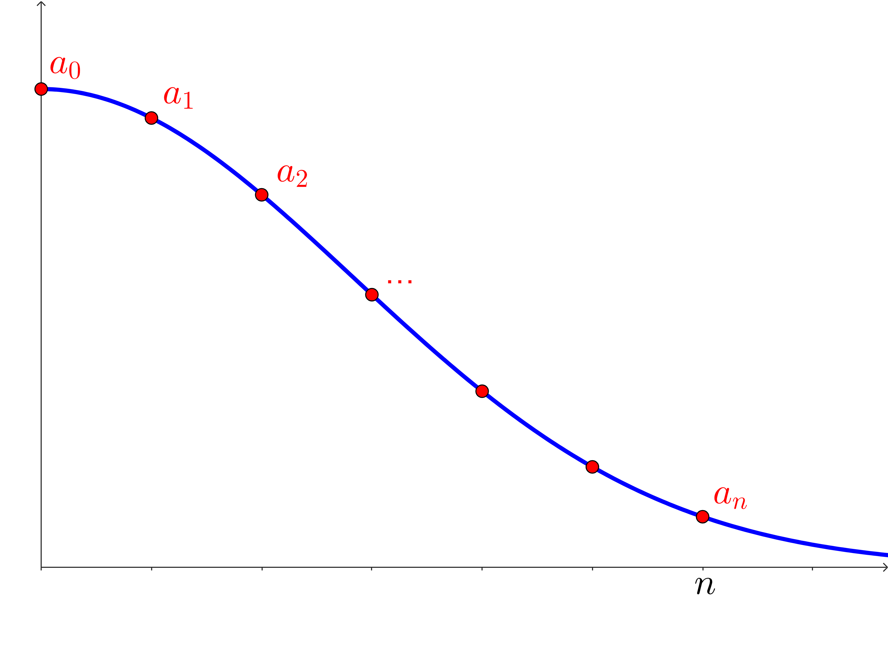
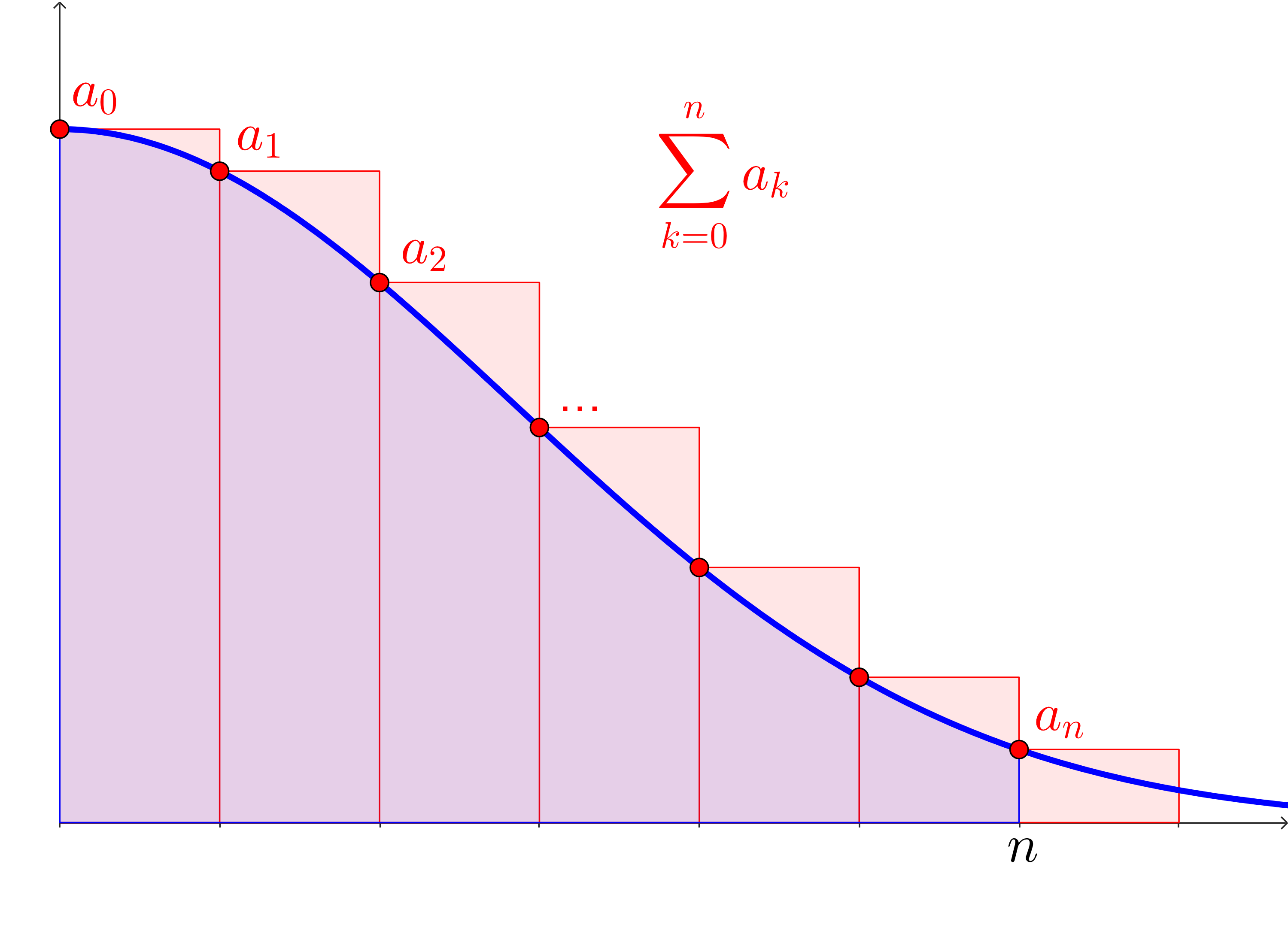
How does the partial sum, $\displaystyle \sum_{k=0}^n a_k$ compare to the Riemann sum for $f(x)$ from $x=0$ to $x=n$ with $n$ rectangles?

🔗

Hint.

It might help to visualize the Left Riemann sum!

🔗

Solution.

Hopefully we can see that the partial sum, $\displaystyle \sum_{k=0}^n a_k$ is the exact same thing as the left Riemann sum!

🔗

(b)

We’re going to visualize the accumulation of $f(x)$ from $x=0$ to $x=n$ by thinking about the integral:

\begin{equation*} \int_{x=0}^{x=n} f(x)\;dx\text{.} \end{equation*}

🔗

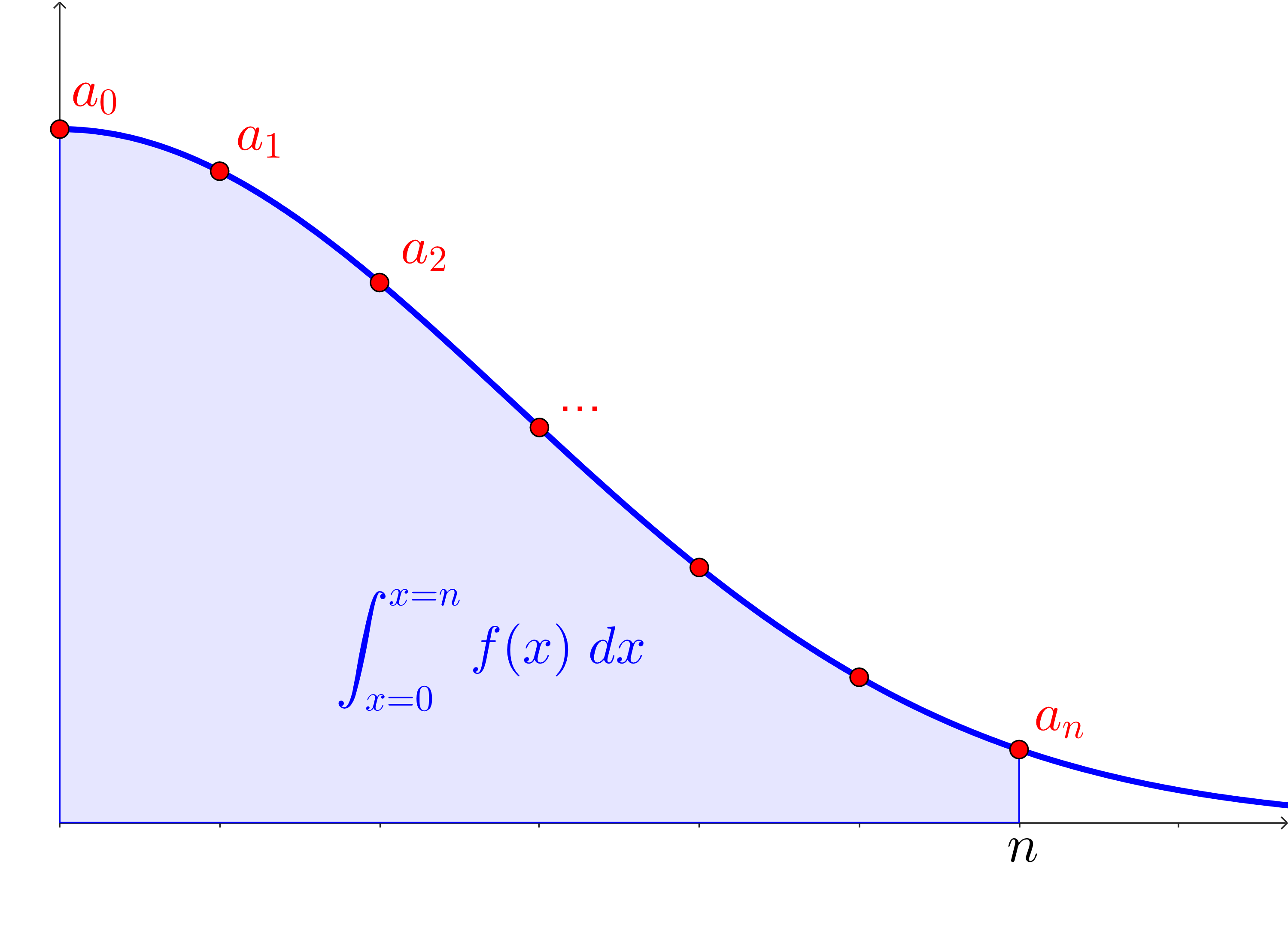
The blue curve, with the area shaded from x=0 to x=n. The area is labeled with the definite integral. — Figure 8.4.4.
🔗

How does this area compare to the Riemann sum you thought of above? Compare them with an inequality and make sure you can explain why this has to be true.

🔗

Hint.

Here’s a picture of the left Riemann sum!

🔗

The left Riemann sum formed at each red point. — Figure 8.4.5.
🔗

🔗

Solution.

Since $\displaystyle \sum_{k=0}^n a_k$ is a left Riemann sum for $f(x)\text{,}$ and since $f(x)$ is decreasing, then we know that each rectangle is formed from the highest point on each subinterval. That means that each rectangle’s area overestimates the area under the curve on that subinterval. Note, also, that since this is a left Riemann sum, the $n$th rectangle is hanging past the end of the definite integral. This means that:

\begin{equation*} \sum_{k=0}^n a_k \gt \int_{x=0}^{x=n} f(x)\;dx\text{.} \end{equation*}

🔗

(c)

Remove the first term of the series, $a_0\text{,}$ and instead think of the sum $\displaystyle \sum_{k=1}^n a_k\text{.}$ Can you still think of this as a Riemann sum to approximate the area from the integral $\displaystyle \int_{x=0}^{x=n} f(x)\;dx\text{?}$

🔗

How does this new Riemann sum compare to the area formed by the integral? Compare them with an inequality and make sure you can explain why this has to be true.

🔗

Hint.

Notice, now, that we need $a_1$ to be the representative height for the first rectangle. How does that change the formation of the rectangles?

🔗

Solution.

We can form a Right Riemann sum! Note that we don’t “overhang” the interval anymore.

🔗

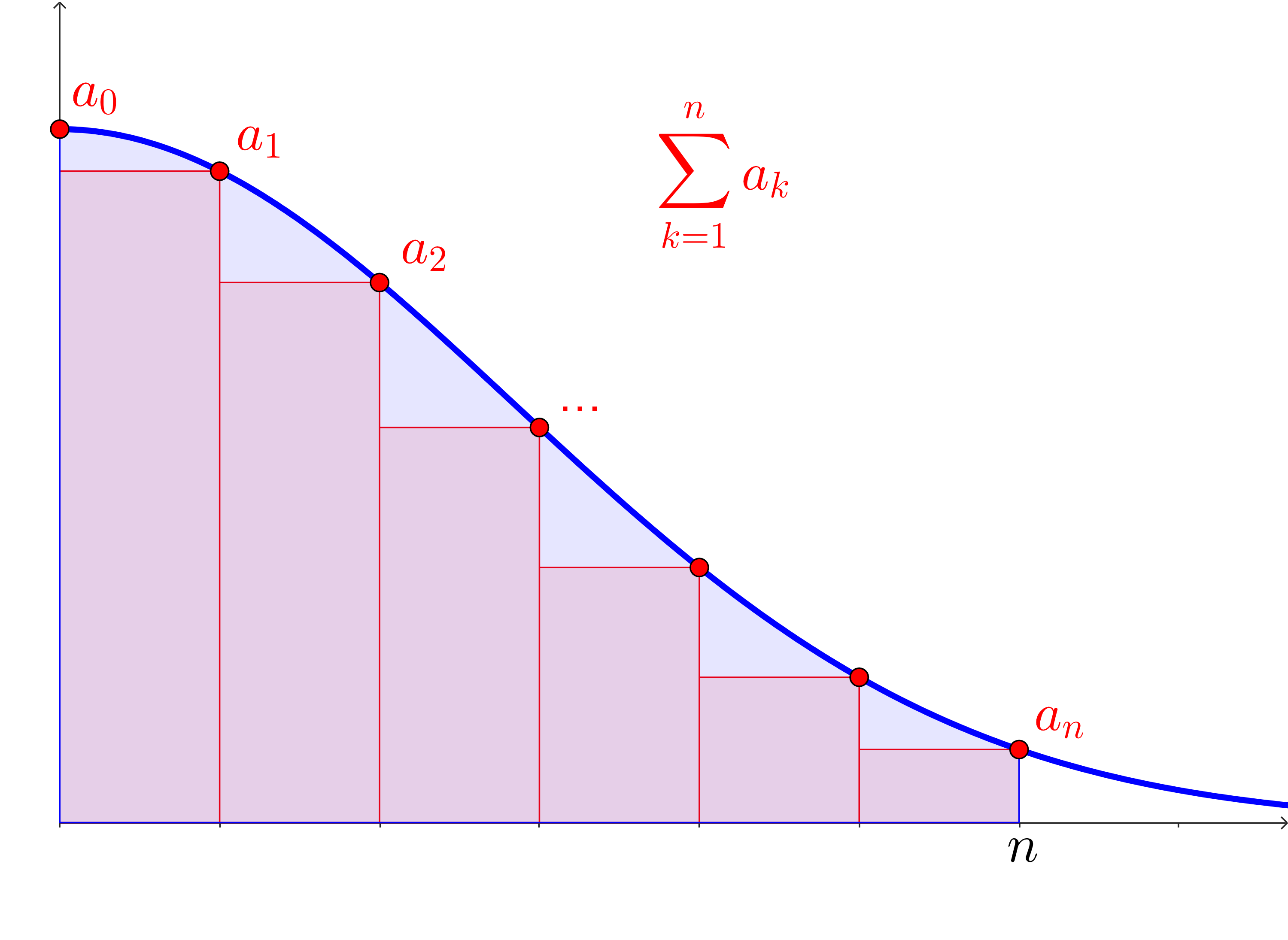
The right Riemann sum formed at each red point, other than the first one. — Figure 8.4.6.
🔗

Note, now, that we are using the lowest point on each subinterval to form the rectangle. This means that:

\begin{equation*} \sum_{k=1}^n a_k \lt \int_{x=0}^{x=n} f(x)\;dx\text{.} \end{equation*}

🔗

(d)

We have thought about two sums, and we can connect them:

\begin{equation*} \sum_{k=0}^n a_k = a_0 + \sum_{k=1}^n a_k\text{.} \end{equation*}

Use the sums to bound the integral:

\begin{equation*} \fillinmath{XXXXXXXX} \lt \int_{x=0}^{x=n} f(x)\;dx \lt \fillinmath{XXXXXXXX} \end{equation*}

🔗

Solution.

\begin{align*} \sum_{k=1}^n a_k \amp \lt \int_{x=0}^{x=n} f(x)\;dx \lt \sum_{k=0}^n a_k \\ \left(\sum_{k=0}^n a_k\right)-a_0 \amp \lt \int_{x=0}^{x=n} f(x)\;dx \lt \sum_{k=0}^n a_k \end{align*}

🔗

(e)

Similarly, use the integral to bound the sum:

\begin{equation*} \fillinmath{XXXXXXXX} \lt \sum_{k=0}^n a_k \lt \fillinmath{XXXXXXXX} \end{equation*}

🔗

Solution.

\begin{equation*} \int_{x=0}^{x=n}f(x)\;dx \lt \sum_{k=0}^n a_k \lt a_0 + \int_{x=0}^{x=n}f(x)\;dx \end{equation*}

🔗

These bounds are going to be super useful! Discovering them is the main task for finding the connections between improper integrals and infinite series. These inequalities might seem kind of strange at first, but we’re going to apply a limit to everything as $n\to \infty\text{,}$ and then think about our definitions of convergence (Definition 7.1.4 and Definition 8.2.2).

🔗

Theorem 8.4.7. Integral Test.

If $\displaystyle\sum_{k=0}^\infty a_k$ is an infinite series with $a_k\gt 0$ for all $k\geq 0$ and $f(x)$ is a continuous and decreasing function with $f(k) = a_k$ for all $k\geq 0\text{,}$ then we can compare the behaviors of $\displaystyle\sum_{k=0}^\infty a_k$ and $\displaystyle\int_{x=0}^\infty f(x)\;dx\text{:}$ the integral and the series are guaranteed to either both diverge or both converge.

🔗

Proof.

The proof of this will come in two parts. First, we’ll prove that $\displaystyle \sum_{k=0}^\infty a_k$ converges when $\displaystyle \int_{x=0}^\infty f(x)\;dx$ converges.

🔗

Then, we’ll prove that $\displaystyle \sum_{k=0}^\infty a_k$ diverges when $\displaystyle \int_{x=0}^\infty f(x)\;dx$ diverges.

🔗

Let’s start with the assumption that $\displaystyle \int_{x=0}^\infty f(x)\;dx$ converges. We know, based on Definition 7.1.4, that this means that $\displaystyle \lim_{n\to\infty} \int_{x=0}^{x=n} f(x)\;dx$ exists. We also know, since $f(x)\gt 0\text{,}$ that

\begin{equation*} \lim_{n\to\infty} \int_{x=0}^{x=n} f(x)\;dx \gt \int_{x=0}^{x=n} f(x)\;dx\text{.} \end{equation*}

This means:

\begin{align*} \sum_{k=0}^n a_k \amp\lt a_0 + \int_{x=0}^{x=n} f(x)\;dx \\ \sum_{k=0}^n a_k \amp \lt a_0 + \lim_{n\to\infty} \int_{x=0}^{x=n} f(x)\;dx \\ \sum_{k=0}^n a_k \amp \lt a_0 + \int_{x=0}^\infty f(x)\;dx \end{align*}

This means that the partial sum, $\displaystyle S_n = \sum_{k=0}^n a_k$ has an upper bound.

🔗

We also know that, since $a_k\gt 0$ for all $k=0,1,2,...\text{,}$ then $S_{n+1}\gt S_n\text{.}$ This means that the sequence of partial sums, $\{S_n\}_{n=0}^\infty$ is both monotonic and bounded, and therefore must converge (by the Monotone Convergence Theorem).
🔗

Thus, $\displaystyle\sum_{k=0}^\infty a_k$ converges.
🔗

🔗
Now, we can start with the assumption that the integral $\displaystyle \int_{x=0}^\infty f(x)\;dx$ diverges. Since we know that $f(x)$ is positive, then we know that

\begin{equation*} \lim_{n\to\infty} \int_{x=0}^{x=n} f(x)\;dx = \infty\text{.} \end{equation*}

We can reconsider the inequalities from Activity 8.4.1:

\begin{align*} \int_{x=0}^{x=n} f(x)\;dx \amp\lt \sum_{k=0}^n a_k \\ \lim_{n\to\infty} \int_{x=0}^{x=n} f(x)\;dx \amp \lt \lim_{n\to\infty} \sum_{k=0}^n a_k\\ \infty \amp\lt \sum_{k=0}^\infty a_k \end{align*}

So then $\displaystyle \sum_{k=0}^\infty a_k$ must also diverge.

🔗

🔗

This is everything we need to prove! Note that we could replicate this proof by swapping the role of the series and the integral to get the same conclusion.

🔗

So now we have a more formal link between these two objects. We have some intuition from Table 8.4.1 that these are pretty similar objects: one of them is an accumulation of function values in a continuous context, while the other is an accumulation of function values in a discrete context.

🔗

We can think about this even more formally! We reminded ourselves at the beginning of this section that, when we think about the limit of a Riemann sum (in the continuous context) that as $n\to\infty\text{,}$ we get $\Delta x \to dx\text{,}$ where $dx$ is essentially the distance between inputs. This produces our integral.

🔗

But now, in the discrete context, we have something different. Without being too formal, we can think about the corresponding limit of $\Delta k$ as we slice this up further. Because our functions are in the discrete context, our inputs have a minimum distance between each other: they’re all 1 unit apart! So here, in the limit where we expect $\Delta x\to dx\text{,}$ we get $\Delta k\to 1\text{.}$ And similarly, in a typical definite integral, we are adding up an infinite number of function outputs between some starting input and stopping input. Now in the discrete context, we don’t get that! We get our normal partial sum:

\begin{equation*} \sum_{k=0}^n a_k \underbrace{\Delta k}_{1} = \sum_{k=0}^n a_k\text{.} \end{equation*}

So the Integral Test is pretty obvious, really: these corresponding objects retain the same type of behavior when we translate them back and forth between the continuous context and the discrete context.

🔗

Great! Let’s apply this, now.

🔗

Example 8.4.8.

For each of the following infinite series, decide whether it is possible (and reasonable) to use the Integral Test. If it is, apply the test and interpret the conclusions.

🔗

(a)

$\displaystyle \sum_{k=0}^\infty \frac{1}{k^2+1}$

🔗

Hint.

This would connect with the integral $\displaystyle \int_{x=0}^\infty \frac{1}{x^2+1}\;dx\text{.}$ Does the function, $f(x)=\dfrac{1}{x^2+1}\text{,}$ meet the requirements of the Integral Test? Does it look like something you could antidifferentiate?

🔗

Solution.

This is a fine opportunity to apply the Integral Test. The Integral Test says that we can link the behavior of the integral and the series:

\begin{equation*} \sum_{k=0}^\infty \frac{1}{k^2+1} \sim \int_{x=0}^\infty \frac{1}{x^2+1}\;dx\text{.} \end{equation*}

Let’s think about the integral!

\begin{align*} \int_{x=0}^\infty \frac{1}{x^2+1}\;dx \amp = \lim_{t\to\infty}\int_{x=0}^{x=t}\frac{1}{x^2+1}\;dx\\ \amp = \lim_{t\to\infty} \left(\tan^{-1}(x)\right)\bigg|_{x=0}^{x=t}\\ \amp = \lim_{t\to\infty}\tan^{-1}(t) - \tan^{-1}(0)\\ \amp = \frac{\pi}{2} - \frac{\pi}{4}\\ \amp = \frac{\pi}{4} \end{align*}

This integral converges.

🔗

Conclusion: Since the integral $\displaystyle \int_{x=0}^\infty \frac{1}{x^2+1}\;dx$ converges, we know that the infinite series $\displaystyle \sum_{k=0}^\infty \frac{1}{k^2+1} $ also converges.

🔗

(b)

$\displaystyle \sum_{k=0}^{\infty} \frac{1}{e^{k^2}}$

🔗

Hint.

We can rewrite $\dfrac{1}{e^{k^2}}$ to $e^{-k^2}\text{,}$ and so we’re thinking about the integral $\displaystyle\int_{x=0}^\infty e^{-x^2}\;dx\text{.}$ Does this function meet the conditions of the Integral Test? Can we antidifferentiate?

🔗

Solution.

Unfortunately, this integral is going to be very difficult for us! The function $f(x)=e^{-x^2}$ has an antiderivative on the interval $[0,\infty)$ (it’s a continuous function, and so it is integrable according to the Fundamental Theorem of Calculus (Part 1)).

🔗

This function, though, doesn’t have what we call an elementary antiderivative: any antideriative of $e^{-x^2}$ can’t be written as a combination of our basic function types.

🔗

This means that we’re unable to integrate this using our typical techniques, and (for now), we don’t know if the integral converges or not.

🔗

Conclusion: We won’t apply the Integral Test, and so we don’t know whether the series $\displaystyle \sum_{k=0}^{\infty} \frac{1}{e^{k^2}}$ converges or not.

🔗

(c)

$\displaystyle \sum_{k=1}^\infty \frac{k}{e^{k^2+1}}$

🔗

Hint.

The Integral Test would connect this series to $\displaystyle \int_{x=1}^{\infty} \frac{x}{e^{x^2+1}}\;dx\text{.}$ Does the function $f(x)=\dfrac{x}{e^{x^2+1}}$ meet the requirements of the Integral Test? Could we antidifferentiate?

🔗

Solution.

Let’s apply the Integral Test. we’ll connect the behavior of the integral and the series:

\begin{equation*} \sum_{k=1}^{\infty} \frac{k}{e^{k^2+1}} \sim \int_{x=1}^\infty \frac{x}{e^{x^2+1}}\;dx\text{.} \end{equation*}

We’ll consider the integral, and use a $u$-substitution where $u=-(x^2+1)$ and $du=-2x\;dx\text{.}$

\begin{align*} \int_{x=1}^\infty \frac{x}{e^{x^2+1}}\;dx \amp = \lim_{t\to\infty} \int_{x=1}^{x=t} \frac{x}{e^{x^2+1}}\;dx\\ \amp = \lim_{t\to\infty} -\frac{1}{2}\int_{x=1}^{x=t} \frac{-2x}{e^{x^2+1}}\;dx\\ \amp = -\frac{1}{2}\lim_{t\to\infty} \int_{u=-2}^{u=-(t^2+1)} e^u\;du\\ \amp = -\frac{1}{2}\lim_{t\to\infty}\left(e^u\right)\bigg|_{u=-2}^{u=-(t^2+1)}\\ \amp = -\frac{1}{2} \lim_{t\to\infty} e^{-t^2+1} - e^{-2}\\ \amp = 0 + \frac{1}{2e^2} \end{align*}

This integral converges.

🔗

Conclusion: The integral $\displaystyle \int_{x=1}^\infty \frac{x}{e^{x^2+1}}\;dx $ converges, and so we know that the infinite series $\displaystyle \sum_{k=1}^{\infty} \frac{k}{e^{k^2+1}}$ also converges.

🔗

(d)

$\displaystyle\sum_{k=2}^{\infty} \frac{1}{k\ln(k)}$

🔗

Hint.

We’re considering the function $f(x)=\dfrac{1}{x\ln(x)}$ and the integral $\displaystyle \int_{x=2}^{\infty} \frac{1}{x\ln(x)}\;dx\text{.}$ Does this work for the Integral Test?

🔗

Solution.

If we apply the Integral Test, we’re connecting the following series and integral:

\begin{equation*} \sum_{k=2}^{\infty} \frac{1}{k\ln(k)} \sim \int_{x=2}^{\infty} \frac{1}{x\ln(x)}\;dx\text{.} \end{equation*}

We’ll consider the integral and use the substitution $u=\ln(x)$ so that $du=\dfrac{1}{x}\;dx\text{.}$

\begin{align*} \int_{x=2}^{\infty} \frac{1}{x\ln(x)}\;dx \amp =\lim_{t\to\infty} \int_{x=2}^{x=t} \frac{1}{x\ln(x)}\;dx\\ \amp = \lim_{t\to\infty} \int_{u=\ln(2)}^{u=\ln(t)} \frac{1}{u}\;du\\ \amp = \lim_{t\to\infty} \left(\ln|u|\right)\bigg|_{u=\ln(2)}^{u=\ln(t)}\\ \amp = \lim_{t\to\infty} \ln|\ln(t)| - \ln(\ln(2))\\ \amp = \infty \end{align*}

This integral diverges.

🔗

Conclusion: We found that the integral $\displaystyle \int_{x=2}^{\infty} \frac{1}{x\ln(x)}\;dx$ diverges, which means that the series $\displaystyle\sum_{k=2}^{\infty} \frac{1}{k\ln(k)}$ also diverges.

🔗

As we develop more strategies and tests for series convergence, we should pause and summarize our test.

🔗

Integral Test Strategy.

We want to use this for functions that are relatively easy to antidifferentiate. Looking for $u$-substitution is a good idea, and sometimes we can straightforwardly apply integration by parts.

🔗

We’ll find, though, that this test will mostly be used to introduce a family of infinite series and build up our intuition about partial sums (since we’re really using the integrals to find a bound on our monotonic sequence of partial sums).

🔗

Subsection Why Do We Need These Conditions?

Before we wrap things up, let’s just add some commentary on the conditions or requirements of the Integral Test. This is really a part of a broader discussion on conditions/requirements in mathematical results in general, but we’ll limit ourselves to just this specific test. There are three conditions that we can consider: positive, decreasing, and continuous.

Positive: We need $f(x)$ and $a_k$ to be positive in order for us to get monotonic sequences. Since we know that $a_k\gt 0\text{,}$ we guarantee ourselves that $S_{n+1}\gt S_n\text{,}$ since we’re really adding another positive term. The same thing is true for the integrals, where we guarantee that

\begin{equation*} \displaystyle \int_{x=0}^{x=n+1} f(x)\;dx \gt \int_{x=0}^{x=n} f(x)\;dx\text{.} \end{equation*}

🔗

🔗
Decreasing: This one serves two purposes. First, we use the direction of the function to get some ideas on how the Left and Right Riemann sum compare to the areas: with a decreasing function, the Left sum will always overestimate the integral while the Right sum will underestimate it.
🔗

We could have just required our function to be monotonic, though, since that would guarantee that one of those Riemann sums overestimated the integral while the other underestimated it: we really don’t care about the order. So why would we need it, specifically, to be decreasing? Easy: if $\{a_k\}$ is positive and increasing, then $\displaystyle\lim_{k\to\infty} a_k \neq 0\text{,}$ and we can just apply the Divergence Test.
🔗

🔗
Continuous: This one is pretty simple. Continuity guarantees that an antiderivative of our function exists on the interval we’re looking at. We might not be able to actually find it easily, but at least we know there is one! Without continuity, we can’t antidifferentiate easily and it doesn’t make sense to think about the integral.
🔗

🔗

🔗

We talked about why it’s nice to have a monotonic sequence of terms, but what happens when they aren’t? Briefly, we can say that there are plenty of examples where the series and the integral may not behave similarly. For an easy to see example, let’s consider the following series:

\begin{equation*} \sum_{k=0}^{\infty} \sin^2(\pi\cdot k)\text{.} \end{equation*}

If we try to think about the corresponding integral, we’re considering:

\begin{equation*} \int_{x=0}^\infty \sin^2(\pi\cdot x)\;dx\text{.} \end{equation*}

Can you see what the problem is? The issue becomes evident when we plot the sequence of terms and the continuous function on the same axes.

🔗

An oscillating, periodic, and positive green function labeled f(x) that touches the x-axis at every integer. These points are red, labeled a_0, a_1, a_2, ... — Figure 8.4.9.
🔗

We can see that if we define the sequence of terms using $a_k=\sin^2(\pi\cdot k)\text{,}$ then $a_k = 0$ for $k=0,1,2,...\text{.}$ This means that

\begin{equation*} \sum_{k=0}^{\infty} \sin^2(\pi\cdot k) = 0 + 0 + 0 + ... = 0\text{.} \end{equation*}

Meanwhile, we can see that the integral $\displaystyle \int_{x=0}^\infty \sin^2(\pi\cdot x)\;dx$ will diverge to $\infty\text{,}$ since every oscillation adds the same positive area over and over. The limit will not exist!

🔗

In the Integral Test, and in general, we want to (and need to) be careful about the conditions we apply: we want them to be general enough that we can actually use the test, but specific enough to protect against strange counter-examples.

🔗

Overall, we’re really just trying to connect an integral in one context to an integral in another context. We have talked, briefly, about how we can think of an infinite series as a kind of improper integral for some discrete function (since we are summing up the function values multiplied by the minimal distance between inputs).

🔗

Earlier (in Section 5.6 Introduction to $u$-Substitution and Section 7.6 Trigonometric Substitution), we tried to visualize the variable substitutions (with Figure 5.6.1, Figure 5.6.2, and Figure 7.6.1) as a translation of functions between one context and another. We can visualize the Integral Test in a similar way: we’re translating our integral from a Discrete context into a Continuous context, figuring out whether the integral converges in this context, and then taking the conclusions and applying them to the integral in the Discrete context.

🔗

$Two rectangles, one labeled "Discrete Context" and the other, beside it, labeled "Continuous Context." Inside the "Discrete Context" rectangle is an infinite series with an arrow pointing towards "Existence of limit of partial sums". Inside the "Continuous Context" rectangle is an improper integral with an arrow pointing towards "Existence of limit of definite integral". There is an arrow connecting the infinite series in the first rectangle to the improper integral. Then there is an arrow connecting the statements about the existence of limits.$

Figure 8.4.10. Integral Test, visualized as a transformation between contexts.

🔗

In both the discrete context and the continuous context, we care about whether the limit of the partial sum (or the limit of the definite integral) exists. Under the conditions of the Integral Test, though, we can translate our infinite series to the continuous context and represent it as a traditional improper integral. If we can get conclusions about whether the improper integral converges or not (based on the behavior of the limit of the definite integral), then we can bring that conclusion back to the discrete context and apply it to the limit of the partial sum.

🔗

This process works both ways! We could use information about an infinite series to learn about whether the corresponding improper integral converges or not! But for now, we are likely much more confident working with the integral in the continuous context, and so it makes most sense to think about the Integral Test using the directions pictured in Figure 8.4.10.

🔗

Practice Problems Practice Problems

1.

What are the conditions of the Integral Test? What are the conclusions of the Integral Test?

🔗

2.

For each of the following series, apply the Integral Test and interpret the conclusion of the test.

🔗

(a)

$\displaystyle\sum_{k=1}^\infty \left(\frac{k}{k^2+1}\right)$

🔗

(b)

$\displaystyle\sum_{k=1}^\infty \left(\frac{k}{e^k}\right)$

🔗

(c)

$\displaystyle\sum_{k=2}^\infty \left( \frac{1}{k\ln(k)} \right)$

🔗

(d)

$\displaystyle\sum_{k=1}^\infty \left( \frac{k^2+k}{e^k} \right)$

🔗

(e)

$\displaystyle\sum_{k=1}^\infty \left( \frac{1}{k^2+1} \right)$

🔗

3.

For what values of $p$ (with $p\gt 0$) will the following series converge?

\begin{equation*} \sum_{k=1}^\infty \frac{1}{k^p} \end{equation*}

🔗

4.

For what values of $r$ (with $r\gt 0$) will the following series converge?

\begin{equation*} \sum_{k=0}^\infty r^k \end{equation*}

🔗

Prev Top Next

Object	Continuous Context	Discrete Context
Function	\(f(x)\)	\(a_k\)
Graph	Figure 8.1.4	Figure 8.1.5
Finite Accumulation	Definite Integral	Partial Sum
	\(\displaystyle A(t) = \int_{x=0}^{x=t} f(x)\;dx\)	\(\displaystyle S_n = \sum_{k=0}^n a_k\)
Infinite Accumulation	Improper Integral	Infinite Series
	\(\displaystyle\int_{x=0}^\infty f(x)\;dx\)	\(\displaystyle\sum_{k=0}^\infty a_k\)