Activity 1.4.1. What Happens When We Divide by 0?
First, let’s make sure we’re clear on one thing: there is no real number that is represented as some other number divided by 0.
When we talk about “dividing by 0” here (and in Section 1.3), we’re talking about the behavior of some function in a limit. We want to consider what it might look like to have a function that involves division where the denominator gets arbitrarily close to 0 (or, the limit of the denominator is 0).
(a)
Remember when, once upon a time, you learned that dividing one a number by a fraction is the same as multiplying the first number by the reciprocal of the fraction? Why is this true?
(b)
What is the relationship between a number and its reciprocal? How does the size of a number impact the size of the reciprocal? Why?
(c)
Consider \(12\div N\text{.}\) What is the value of this division problem when:
-
\(N=6\text{?}\)
-
\(N=4\text{?}\)
-
\(N=3\text{?}\)
-
\(N=2\text{?}\)
-
\(N=1\text{?}\)
(d)
Let’s again consider \(12\div N\text{.}\) What is the value of this division problem when:
-
\(N = \frac{1}{2}\text{?}\)
-
\(N= \frac{1}{3}\text{?}\)
-
\(N=\frac{1}{4}\text{?}\)
-
\(N=\frac{1}{6}\text{?}\)
-
\(N=\frac{1}{1000}\text{?}\)
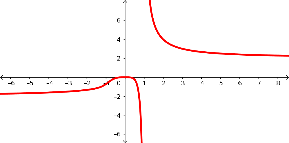
(e)
Consider a function \(f(x) = \frac{12}{x}\text{.}\) What happens to the value of this function when \(x\to 0^+\text{?}\) Note that this means that the \(x\)-values we’re considering most are very small and positive.
(f)
Consider a function \(f(x) = \frac{12}{x}\text{.}\) What happens to the value of this function when \(x\to 0^-\text{?}\) Note that this means that the \(x\)-values we’re considering most are very small and negative.