
Section 6.3 Volumes of Solids of Revolution

Hopefully, by now we’re feeling pretty comfortable with the use of a Riemann sum to create an integral formula. So far, these integral formulas have matched with our intuition somewhat. We probably can justify the integral formula for displacement of an object (Definition 6.1.3 Displacement of an Object) by thinking about the fact that position is an antiderivative of velocity. We probably can convince ourselves about the integral formula for the area between curves (Definition 6.2.5 Area Between Curves) by thinking about subtracting areas, geometrically.
We’re going to make a jump from a 2-dimensional measurement of size, area, to a 3-dimensional measurement of size, volume.

Subsection From Area To Volume

Here’s the basic idea, in a broad overview: if we want to calculate a volume, then we are going to be working with a 3-dimensional solid. We’ll use the slice-and-sum process:
  1. Slice the object into uniformly thick slices along some axis.
  2. For each slice, we’ll approximate the volume. We can do this by thinking about the cross-sectional area. If we assume that the area is constant all the way through the slice (in the same way that we assumed earlier that the heights of our rectangles were constant), then we simply can multiply the cross-sectional area by the thickness to get the volume of each slice:
    \begin{equation*} V_k = A(x_k^*)\Delta x\text{.} \end{equation*}
  3. Approximate the total volume of the solid by adding the volumes of the slices together:
    \begin{equation*} V \approx \sum_{k=1}^n A(x_k^*)\Delta x\text{.} \end{equation*}
  4. Apply a limit, where the number of slices gets infinitely big (and the thickness of each slice gets infinitely small):
    \begin{align*} V \amp = \lim_{n\to\infty}\sum_{k=1}^n A(x_k^*)\Delta x\\ \amp = \int_{x=a}^{x=b} A(x)\;dx \end{align*}
    Here, \(a\) and \(b\) are the \(x\)-values that define the interval we’re slicing along and \(A(x)\) is a formula for the cross-sectional area of the object at \(x\text{.}\)
The biggest issue here is going to be thinking about that formula for area. In order for us to do that, we’re going to think about a specific type of 3-dimensional solid, built in a systematic way so that we can find the cross-sectional areas easily.

Subsection Solids of Revolution

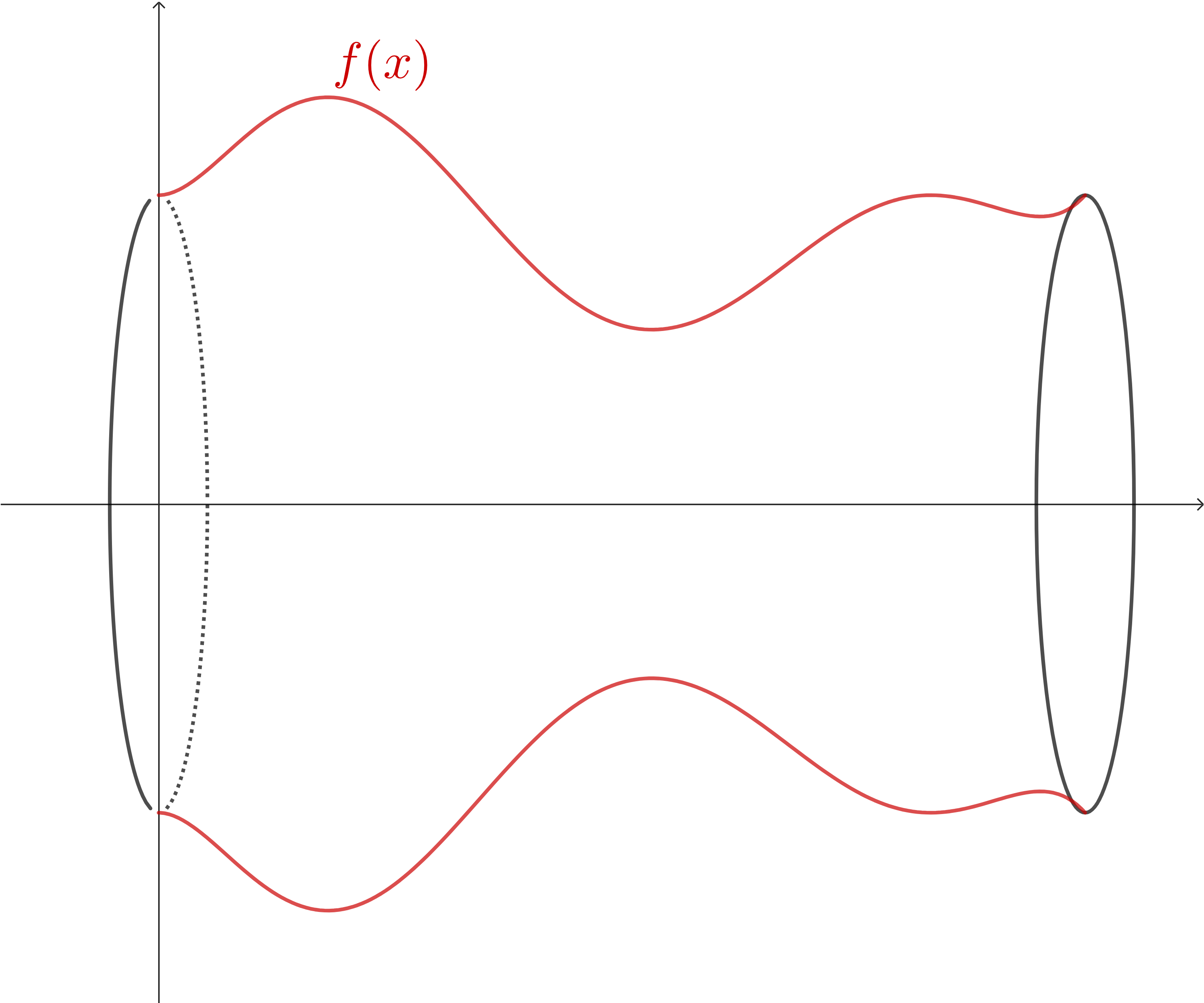
A solid of revolution is a strange type of solid: we’re going to define it based on a 2-dimensional region (we’ll use functions in a normal \(xy\)-plane) that we then imagine revolving around a straight line axis. Maybe we define some region in the upper half of the plane, but then revolve it around the \(x\)-axis. While we imagine this revolution, we want to think about the three dimensional solid that gets "traced" by the curve spinning around the axis. Let’s dive into an example to see.
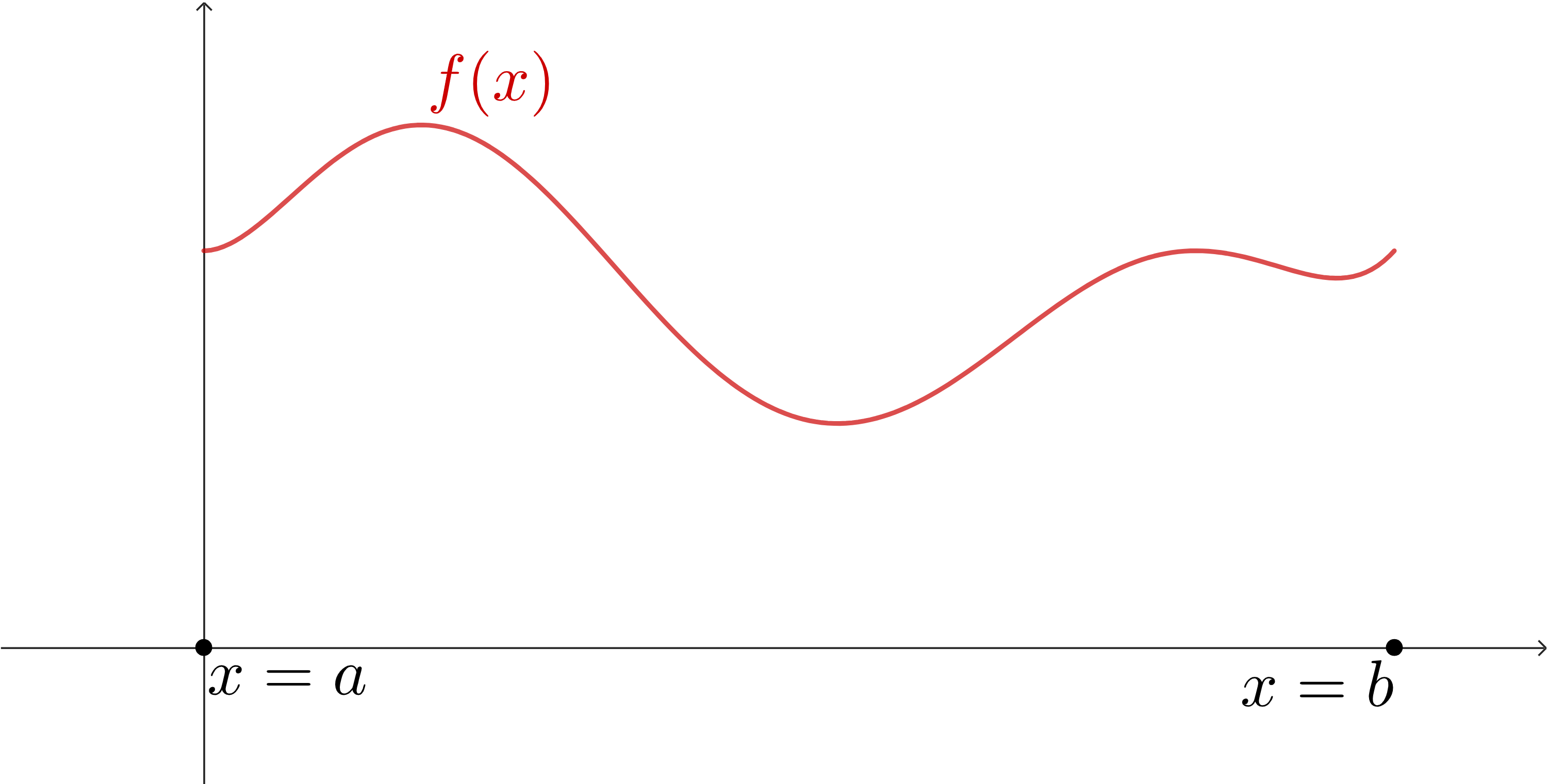
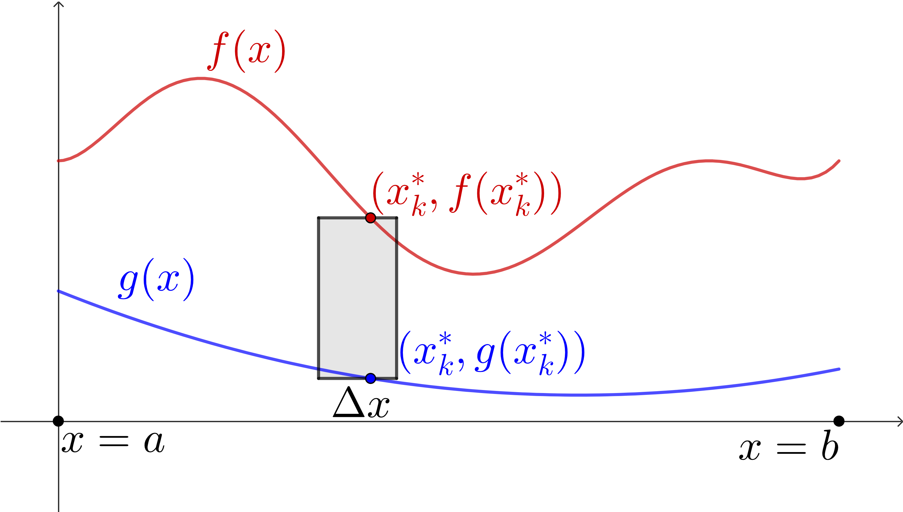
Let’s visualize some function \(f(x)\) defined (and continuous) on the interval \([a,b]\) and with \(f(x)\geq 0\) on that interval. We’ll see why this is useful, but for now, we’re just thinking of some function.
A graph of a red curve labeled f(x). The curve is above the x-axis and starts at the y-axis, and moves forward until it stops. There is are two points on the x-axis labeled x=a and x=b, representing the beginning and ending of the interval where this function is defined. The function looks like a sort of curvy polynomial, and the shape is unimportant.
Figure 6.3.1.
We’re going to revolve this curve (and the region bounded between it and the \(x\)-axis) around the \(x\)-axis. This will create the following shape.
The red curve, f(x), has been revolved around the x-axis. There is a reflection of this curve below the axis, and lines connecting the ends so that the shape looks like a vase on its side, where the outline of the vase is shaped like the graph f(x).
Figure 6.3.2.
So our goal is to find the volume of this type of solid. The curve defining the edge of it can change, but the way that we create it will be systematic enough that we can build a formulaic integral expression for it.
As you would imagine, we’ll start with a rectangle.
A graph of a red curve labeled f(x). The curve is above the x-axis and starts at the y-axis, and moves forward until it stops. There is are two points on the x-axis labeled x=a and x=b, representing the beginning and ending of the interval where this function is defined. The function looks like a sort of curvy polynomial, and the shape is unimportant. There is a red rectangle spanning from the x-axis to the curve, touching the curve at a point labeled (x_k^*, f(x_k^*)). The width of the rectangle is labeled Delta x.
Figure 6.3.3.
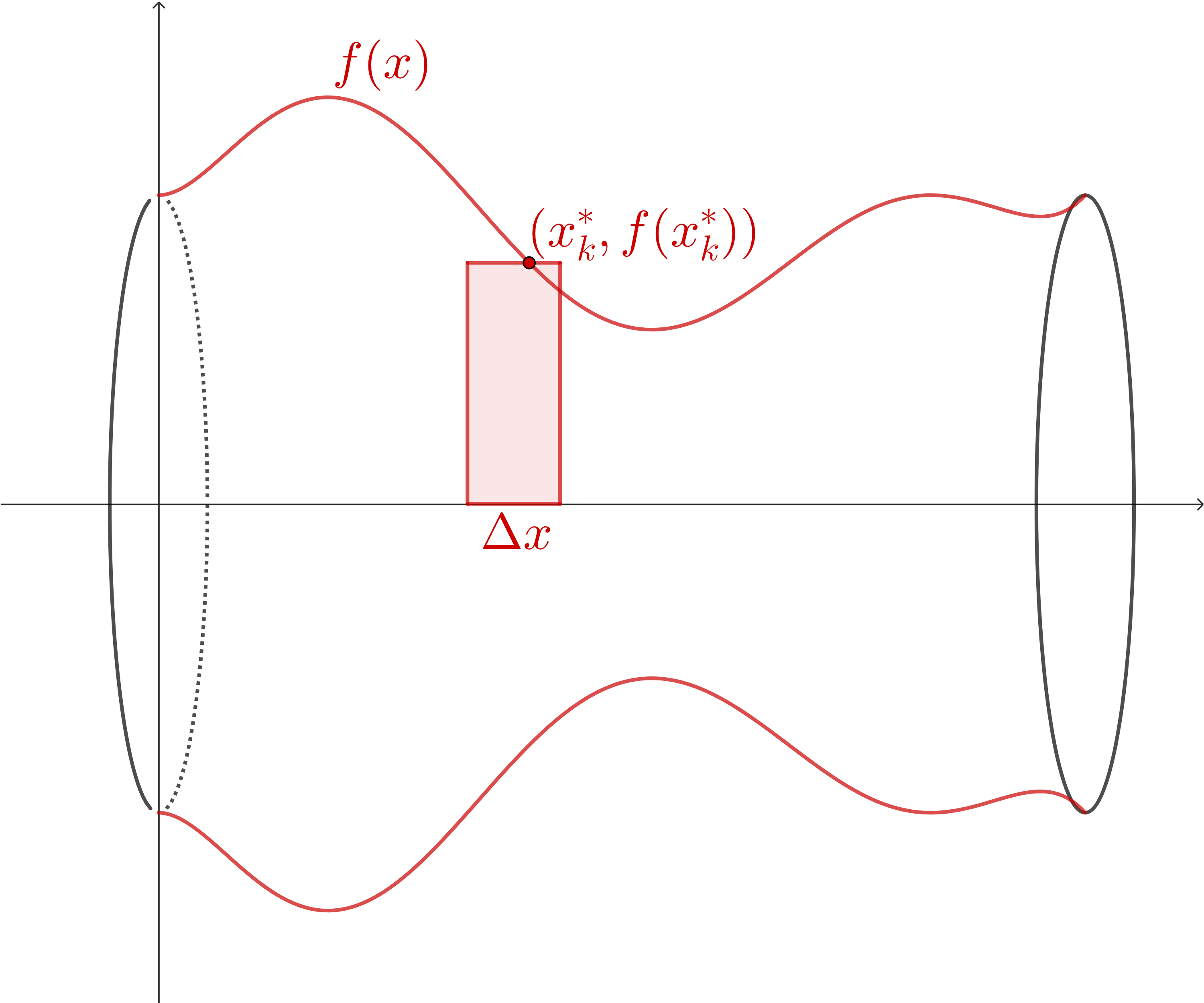
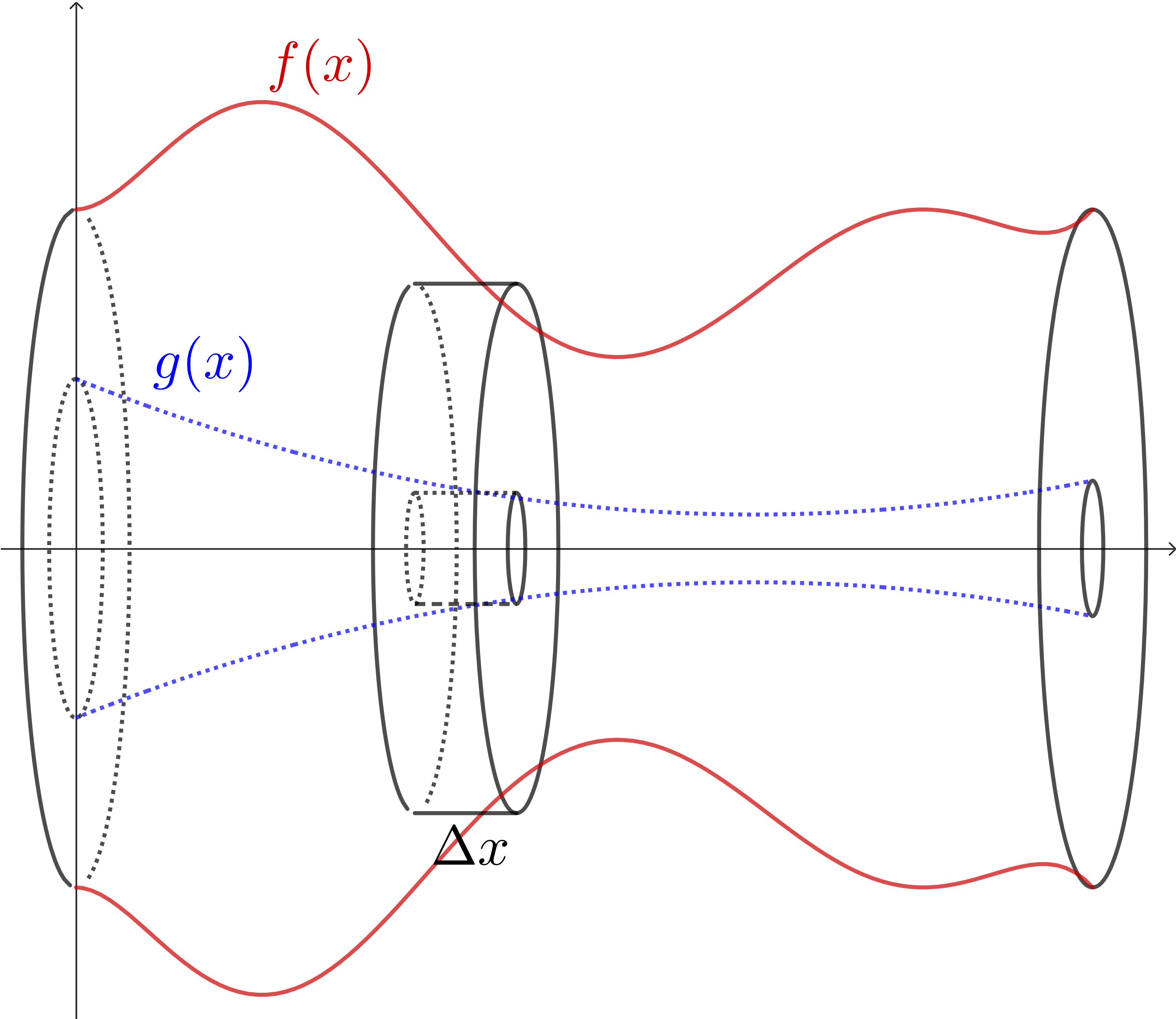
This rectangle will represent a single, generic slice. We really want to imagine a slice of the 3-dimensional solid, though, and so we will revolve this rectangle around the \(x\)-axis. This will create a slice of our solid of revolution. From there, we can think about the volume of this generic \(k\)th slice, and fall into the rhythm of our slice-and-sum process.
The red curve, f(x), has been revolved around the x-axis. There is a reflection of this curve below the axis, and lines connecting the ends so that the shape looks like a vase on its side, where the outline of the vase is shaped like the graph f(x). Somewhere in the middle of the vase is a sliced region, looking like a small coin. This is the rectangle, revolved around the axis. The point on the curve is still labeled (x_k^*, f(x_k^*)) and the width of this slice is labeled Delta x.
Figure 6.3.4.
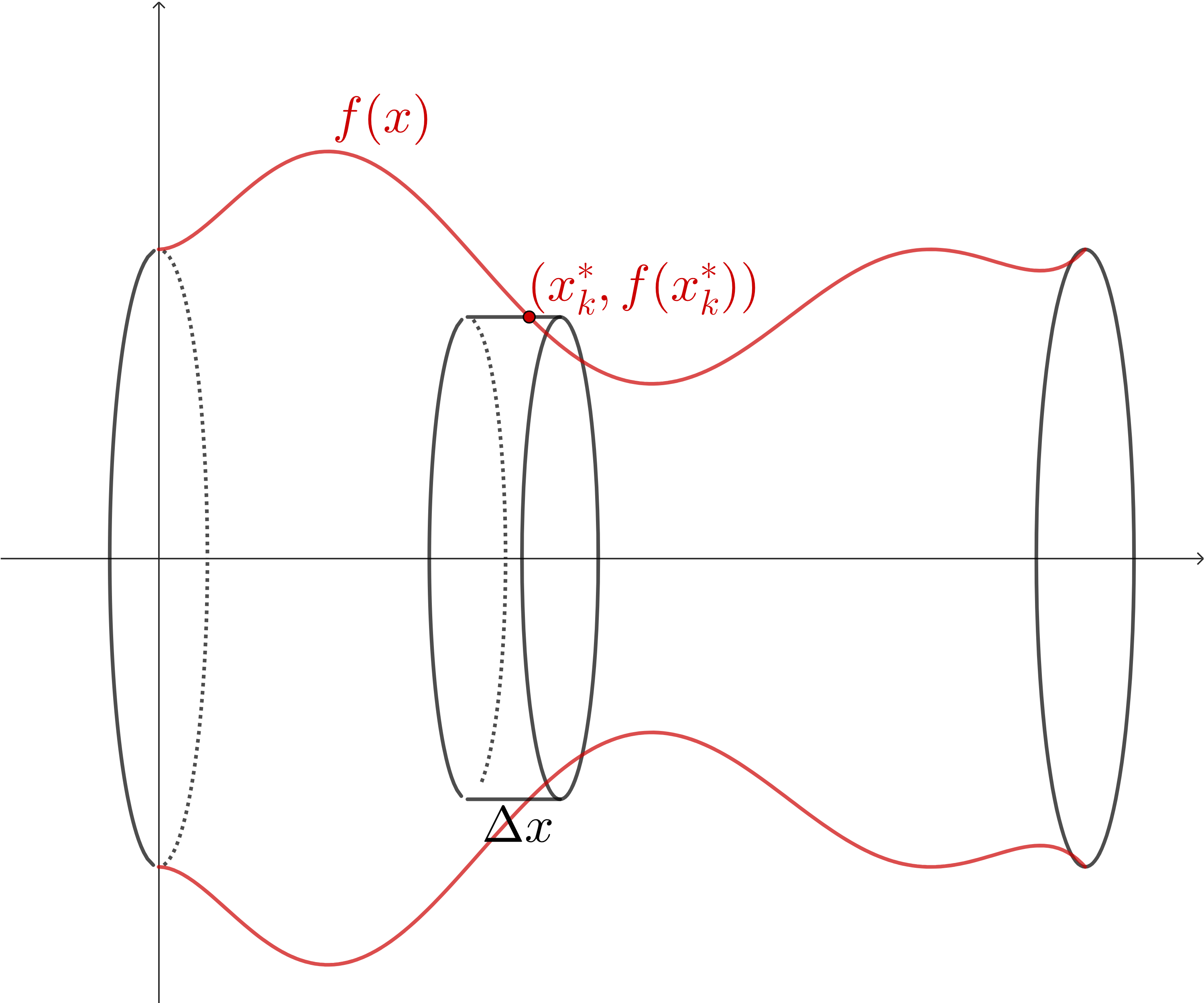
We want to find the volume of this specific slice. To do this, we can remove this stubby cylinder from the solid and think about it directly. We can see the thickness of the slice is represented by \(\Delta x\text{,}\) and so we need to think about the cross-sectional area of the "face" of this slice.
A circle where the radius is labeled r=f(x_k^*).
Figure 6.3.5.
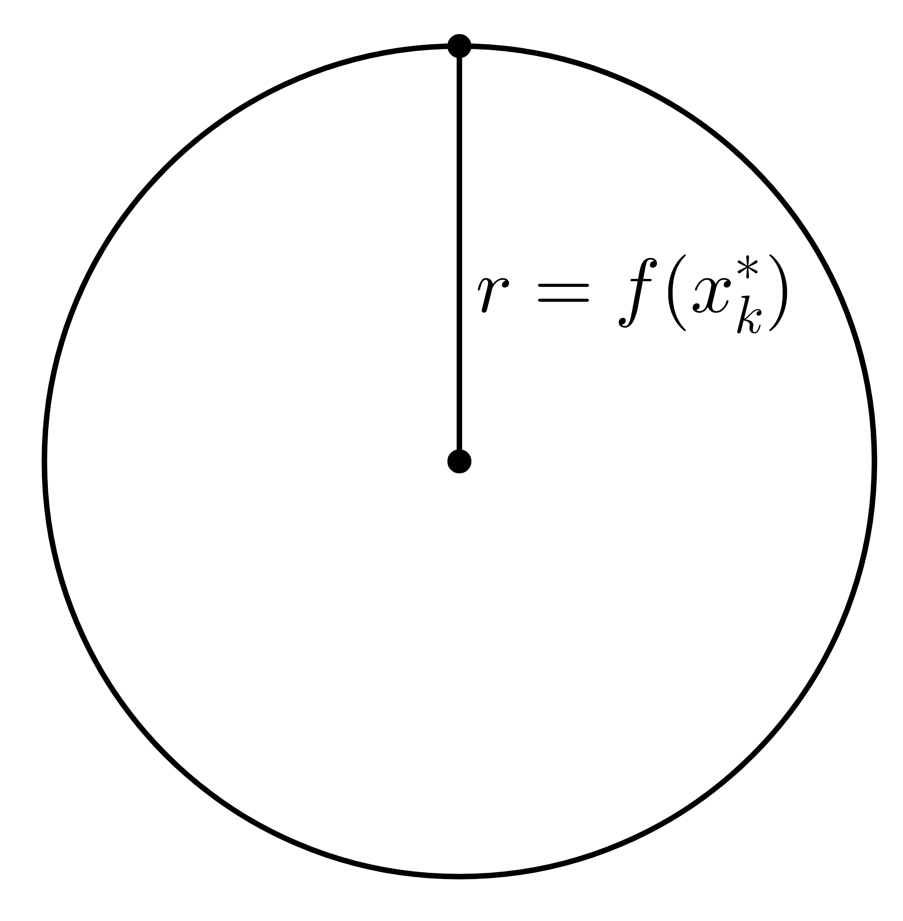
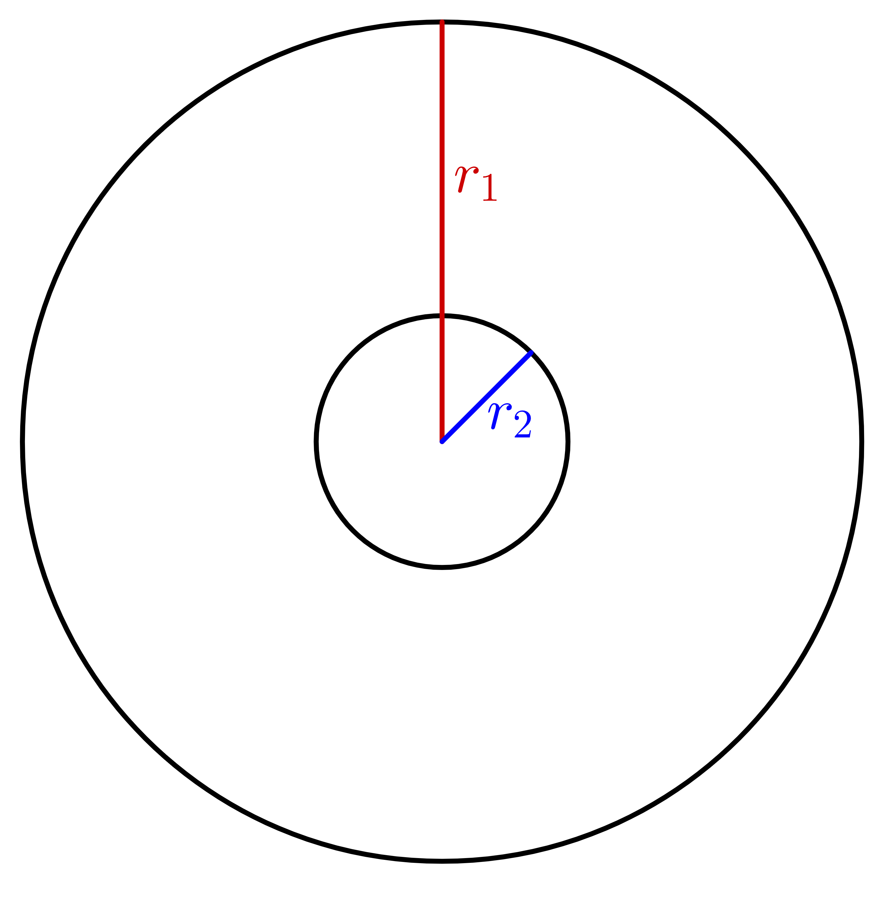
This is something we easily can find the area of! We know the formula for the area of a circle: \(A=\pi r^2\text{.}\) We’ll notice that the radius of this circle is the distance from the center of our slice to the outer edge: this is the height of the rectangle in Figure 6.3.3. So we can use \(r=f(x_k^*)\text{,}\) giving us the cross-sectional area of the \(k\)th slice:
\begin{equation*} A(x_k^*) = \pi \left(f(x_k^*)\right)^2\text{.} \end{equation*}
Now, we can drop into our slice and sum process:
  1. The volume of the \(k\)th slice is:
    \begin{align*} V_k \amp = A(x_k^*) \Delta x\\ \amp = \pi\left(f(x_k^*)\right)^2 \Delta x \end{align*}
  2. We can approximate the volume by adding the slices:
    \begin{equation*} V \approx \sum_{k=1}^n \pi\left(f(x_k^*)\right)^2 \Delta x \end{equation*}
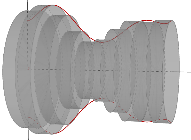
    Sometimes this can be hard to visualize. We’re approximating the solid in Figure 6.3.2 by thinking about a bunch of these circular disks stacked next to each other.
    The 3-dimensional solid, but there are 10 grey circular disks stacked next to each other. The radius of each varies, matching with the curve outlining the vase-like image.
    Figure 6.3.6.
  3. We can apply a limit to evaluate the actual volume of the solid and construct a definite integral.
    \begin{align*} V \amp = \lim_{n\to\infty} \sum_{k=1}^n \pi\left(f(x_k^*)\right)^2 \Delta x\\ \amp = \int_{x=a}^{x=b} \pi (f(x))^2\;dx \end{align*}
This is great! We’ll call this volume integral the Disk Method, since each cross section is a circular disk.
What happens if we add a second curve defining a lower boundary to the region, like we did in Section 6.2 Area Between Curves for areas?

Activity 6.3.1. Carving out a Hole in the Center.

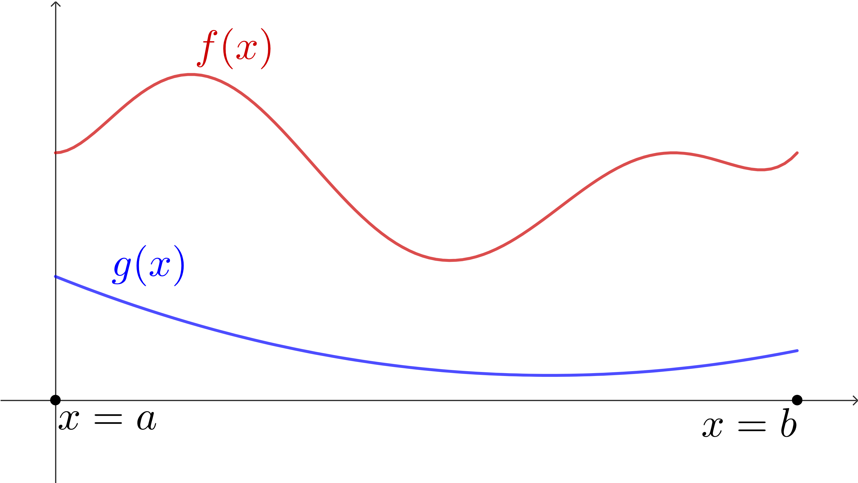
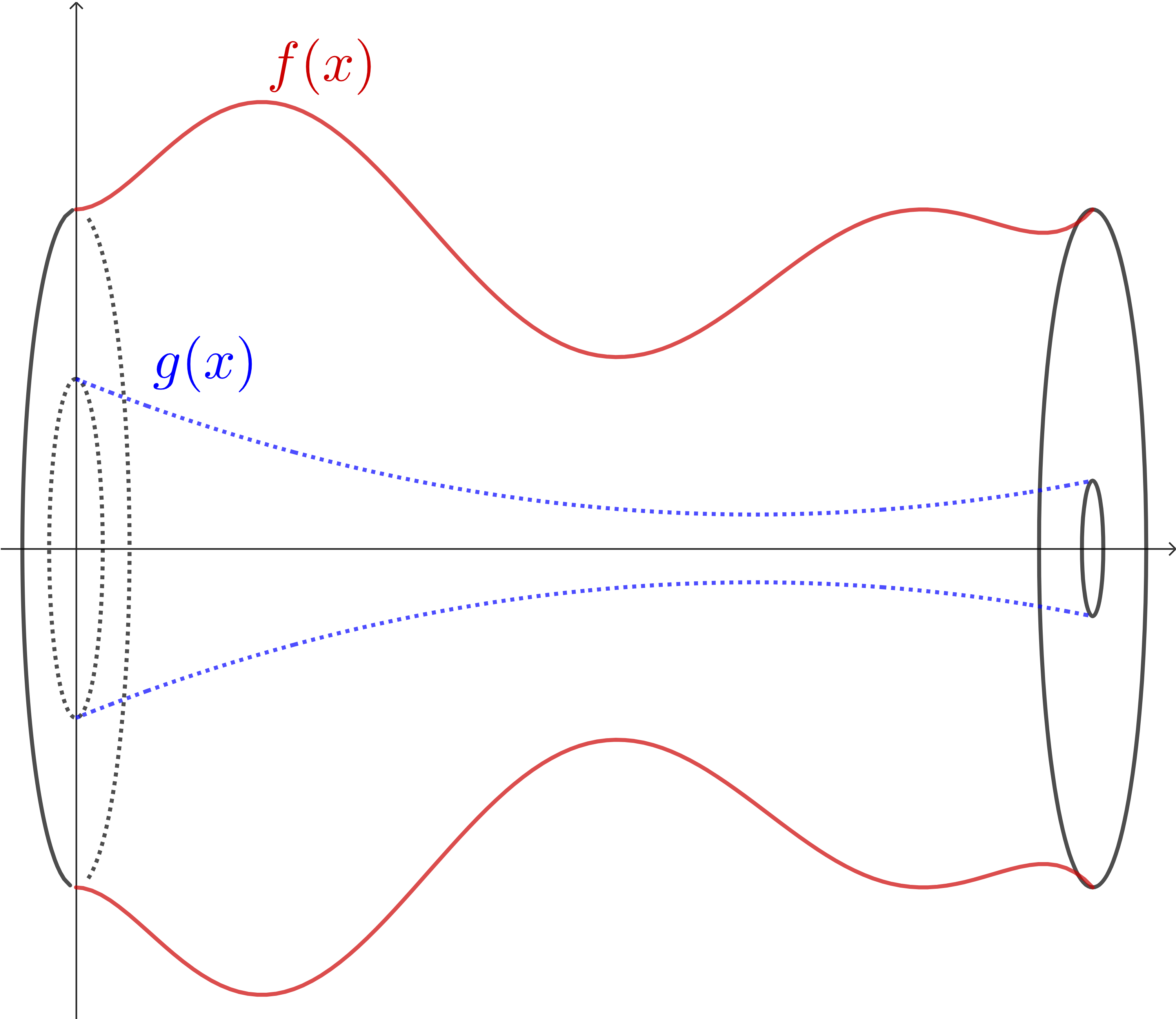
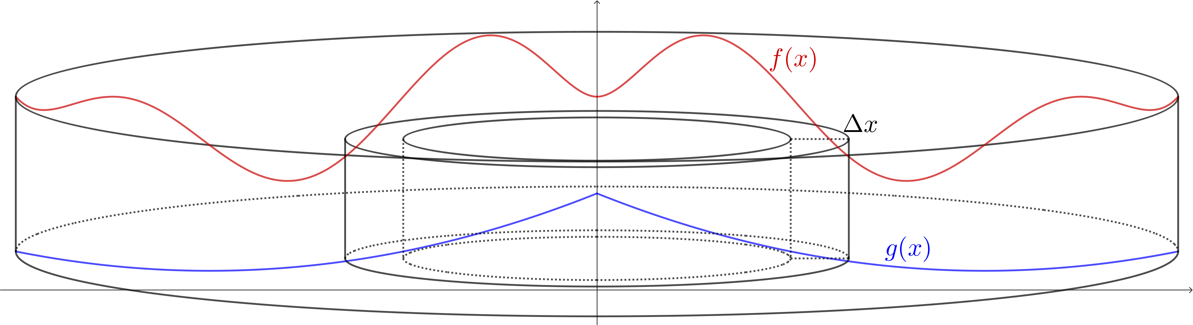
We’re going to look at the same solid as in Figure 6.3.2. But this time, when we define the 2-dimensional region that we’re going to revolve around the \(x\)-axis, we’re going to add a lower boundary function, \(g(x)\text{.}\)
A graph of two functions. The upper function is red, labeled f(x), and is a wavy polynomial. It is above the second function, g(x), which is blue. It is less wavy. Both of them are above the x-axis, and go from a point labeled x=a to x=b where they both stop.
Figure 6.3.7.
When we revolve this region around the \(x\)-axis, we get the following 3-dimensional solid.
The region revolved around the x-axis. It creates a vase type shape where the outer edge is the red f(x) function on the top and reflected onto the bottom. The inner function, g(x), creates a kind of tunnel through the solid.
Figure 6.3.8.
(a)
How is a single generic slice on this solid different than the one in Figure 6.3.2?
Hint 1.
Here is the rectangle that will define that slice!
A graph of two functions. The upper function is red, labeled f(x), and is a wavy polynomial. It is above the second function, g(x), which is blue. It is less wavy. Both of them are above the x-axis, and go from a point labeled x=a to x=b where they both stop. A rectangle spans from the bottom g(x) function to the top f(x) function, with the point on the bottom labeled (x_k^*, g(x_k^*)) and the point on the top labeled (x_k^*, f(x_k^*)). The width of the rectangle is labeled Delta x.
Figure 6.3.9.
Hint 2.
Here is the slice formed when the rectangle revolves around the axis!
The region revolved around the x-axis. It creates a vase type shape where the outer edge is the red f(x) function on the top and reflected onto the bottom. The inner function, g(x), creates a kind of tunnel through the solid. There is a disk with a hole in it, sliced in the middle of the solid. The width is labeled Delta x. The outer edge of the disk matches the function f(x) and the hole is formed from g(x).
Figure 6.3.10.
(b)
Find a formula for the area of the face of the cross-sectional slice.
Hint.
Here’s a picture of the face of the slice!
A circle within a circle. The larger circle has a red radius, labeled r_1. The smaller circle has a blue radius, labeled r_2.
Figure 6.3.11.
Solution.
\begin{align*} A \amp = \pi r_1^2 - \pi r_2^2\\ A(x_k^*) \amp = \pi \left(f(x_k^*)\right)^2 - \pi\left(g(x_k^*)\right)^2 \end{align*}
(c)
Use the slice-and-sum process to create an integral expression representing the volume of this solid.
Solution.
\begin{align*} V_k \amp= \left(\pi \left(f(x_k^*)\right)^2 - \pi\left(g(x_k^*)\right)\right)\Delta x \\ \amp = \pi\left((f(x_k^*))^2-(g(x_k^*))^2\right)\Delta x\\ V \amp \approx \sum_{k=1}^n \pi\left((f(x_k^*))^2-(g(x_k^*))^2\right)\Delta x\\ V \amp = \lim_{n\to\infty} \sum_{k=1}^n \pi\left((f(x_k^*))^2-(g(x_k^*))^2\right)\Delta x\\ \amp = \int_{x=a}^{x=b} \pi\left((f(x))^2-(g(x))^2\right)\;dx \end{align*}

Definition 6.3.12. Volume by Disks/Washers.

If \(f\) and \(g\) are continuous functions with \(f(x)\geq g(x) \geq 0\) on the interval \([a,b]\text{,}\) then the volume of the solid formed by revolving the region bounded between the curves \(y=f(x)\) and \(y=g(x)\) from \(x=a\) to \(x=b\) around the \(x\)-axis is:
\begin{equation*} V = \pi\int_{x=a}^{x=b}\left( (f(x))^2 - (g(x))^2 \right)\;dx\text{.} \end{equation*}
This is called the Washer Method. Note that if \(g(x) = 0\text{,}\) then the resulting volume is:
\begin{equation*} V = \pi\int_{x=a}^{x=b}\left(f(x)\right)^2\;dx\text{.} \end{equation*}
This is called the Disk Method.
We’ll walk through two examples where we construct these integral expressions before pretending to be too comfortable. Let’s start with something similar to what we’ve just done.

Activity 6.3.2. Volumes by Disks/Washers.

Consider the region bounded between the curves \(y=4+2x-x^2\) and \(y=\dfrac{4}{x+1}\text{.}\) We will create a 3-dimensional solid by revolving this region around the \(x\)-axis.
Graph of the region bounded between the parabola y=4+2x-x^2 and the curve y=4/(x+1). The curves intersect at (0,4) and at (3,1), and the parabola defines the top of the region. The whole region is above the x-axis.
Figure 6.3.13.
(a)
Visualize the solid you’ll create when you revolve this region around the \(x\)-axis.
(b)
Draw a single rectangle in your region, standing perpendicular to the \(x\)-axis.
(c)
Let’s use this rectangle to visualize the \(k\)th slice of this 3-dimensional solid. What does the "face" of it look like?
Hint.
It should be a circle within a circle like in Figure 6.3.11, but can you be more detailed with labeling the radii?
(d)
Find the area of the face of the \(k\)th slice.
Hint.
Note that this is a 2-dimensional shape, and we’re just finding the area of it.
Answer.
\(A(x_k^*) = \pi\left((4+2x_k^*-(x_k^*)^2)^2 - \left(\frac{4}{x_k^*+1}\right)^2\right)\)
(e)
Set up the integral representing the volume of the solid.
Hint.
The sum is going to be adding up all of the areas multiplied by \(\Delta x\text{.}\) What will that look like in the integral?
Solution.
\begin{align*} V \amp = \lim_{n\to\infty}\sum_{k=1}^n \pi\left((4+2x_k^*-(x_k^*)^2)^2 - \left(\frac{4}{x_k^*+1}\right)^2\right)\Delta x\\ \amp = \pi \int_{x=0}^{x=3}\left((4+2x-x^2)^2 - \left(\frac{4}{x+1}\right)^2\right)\;dx \end{align*}
(f)
Can you describe how you would antidifferentiate and evaluate this integral?
Hint.
What happens when you square these functions? What kinds of strategies will you use for the types of functions you’re left with?
Solution.
The first function, the quadratic, will be annoying to square. We’ll end up with some big degree 4 polynomial, though, and antidifferentiating will be easy, since we can use the Power Rule.
The second function squared will give us \(\dfrac{4}{(x+1)^2}\text{.}\) We can use a \(u\)-substitution here with \(u=x+1\text{.}\) Then, we have a negative exponent and we can use the Power Rule!
Ok, so when we’re creating these integrals, we really are focussing on using the rectangle we drew to show us which functions serve as the large radius compared to the small radius. In the next example, we’ll see another key thing to notice from a single rectangle.

Activity 6.3.3. Another Volume.

Now let’s consider another region: this time, the one bounded between the curves \(y=x\) and \(y=3\sqrt{x}\text{.}\) We will, again, create a 3-dimensional solid by revolving this region around the \(y\)-axis.
Graph of the region bounded between the root function y=3sqrt(x) and the line y=x. The curves intersect at (0,0) and at (9,9), and the root defines the top of the region. The whole region is above the x-axis.
Figure 6.3.14.
(a)
Visualize the solid you’ll create when you revolve this region around the \(y\)-axis.
(b)
Draw a single rectangle in your region standing perpendicular to the \(y\)-axis.
Hint.
Notice that your rectangle is sitting on its side now! This will change some things for us in a familiar way!
(c)
Let’s use this rectangle to visualize the \(k\)th slice of this 3-dimensional solid. What does the "face" of it look like?
Hint.
It should be a circle within a circle like in Figure 6.3.11, but can you be more detailed with labeling the radii?
(d)
Find the area of the face of the \(k\)th slice.
Hint.
Note that this is a 2-dimensional shape, and we’re just finding the area of it. You’ll also notice that the radii are measuring a horizontal distance in terms of a differing height, so you’ll want to express these as functions of \(y\text{.}\)
Solution.
The outer radius comes from the function \(y=x\text{,}\) but we’ll invert it to be \(x=y\text{.}\)
The inner radius comes from the function \(y=3\sqrt{x}\text{,}\) but we’ll invert it be written as \(x=\left(\dfrac{y}{3}\right)^2\) or \(x=\dfrac{y^2}{9}\text{.}\)
\begin{equation*} A(y_k^*) = \pi\left((y_k^*)^2 - \left(\frac{(y_k^*)^2}{9}\right)^2\right) \end{equation*}
(e)
Set up the integral representing the volume of this solid.
Solution.
\begin{align*} V \amp = \lim_{n\to\infty} \sum_{k=1}^n \pi\left((y_k^*)^2 - \left(\frac{(y_k^*)^2}{9}\right)^2\right) \Delta y\\ \amp =\pi\int_{y=0}^{y=9} y^2-\frac{y^4}{81}\;dy \end{align*}
Notice that the rectangle was the clue that we were going to be using \(\Delta y\) when we calculated volumes. This ended up being the reason that we integrated with regard to \(y\text{,}\) since the \(\Delta y\to dy\) in the integral.
A single rectangle, carefully drawn, can give us a large amount of information as we try to juggle these volumes!

Subsection Reorienting our Rectangles

We saw in Activity 6.3.3 that thinking about the single rectangle we drew was helpful. We’ll see that again in this next formula that we build.
Notice that, in all of the previous work we’ve done, we’ve drawn our rectangle so that it is standing perpendicular to the axis of revolution. This is the kind of rectangle that, when we revolve it, traces out the "washer" shape!
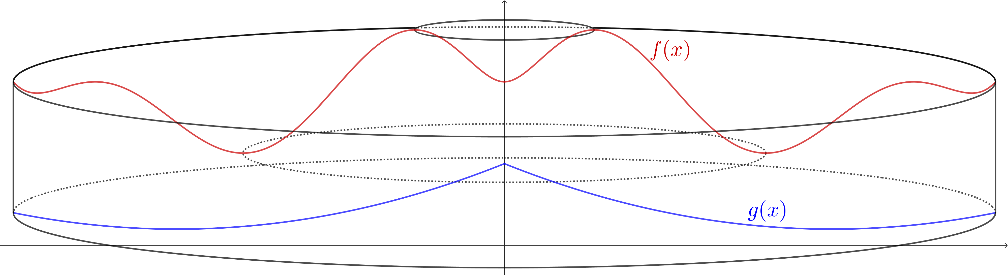
So what happens when we change the orientation of our rectangle? What happens when we draw a rectangle that is parallel to the axis of revolution? Let’s consider the same region as before (the one we visualized in Figure 6.3.7) with the same rectangle as before (the one we visualized in Figure 6.3.9), but we’ll revolve around the \(y\)-axis.
When we revolve this region around the \(y\)-axis, we end up with the following solid.
A cylindrical looking solid, where the top of the solid is formed by the red f(x) function and its reflection across the y-axis, while the bottom is formed by the blue g(x) and its reflection. Some circles are also marked, showing the shape of the top.
Figure 6.3.15.
We want to focus on the single rectangle and the shape that it forms when we revolve it around the \(y\)-axis. From there, we can fall into our slice and sum process by thinking about how we might calculate the volume of this single sliced piece and then adding them up.
A cylindrical looking solid, where the top of the solid is formed by the red f(x) function and its reflection across the y-axis, while the bottom is formed by the blue g(x) and its reflection. Some circles are also marked, showing the shape of the top. A single rectangle and the small cylinder it forms is highlighted.
Figure 6.3.16.
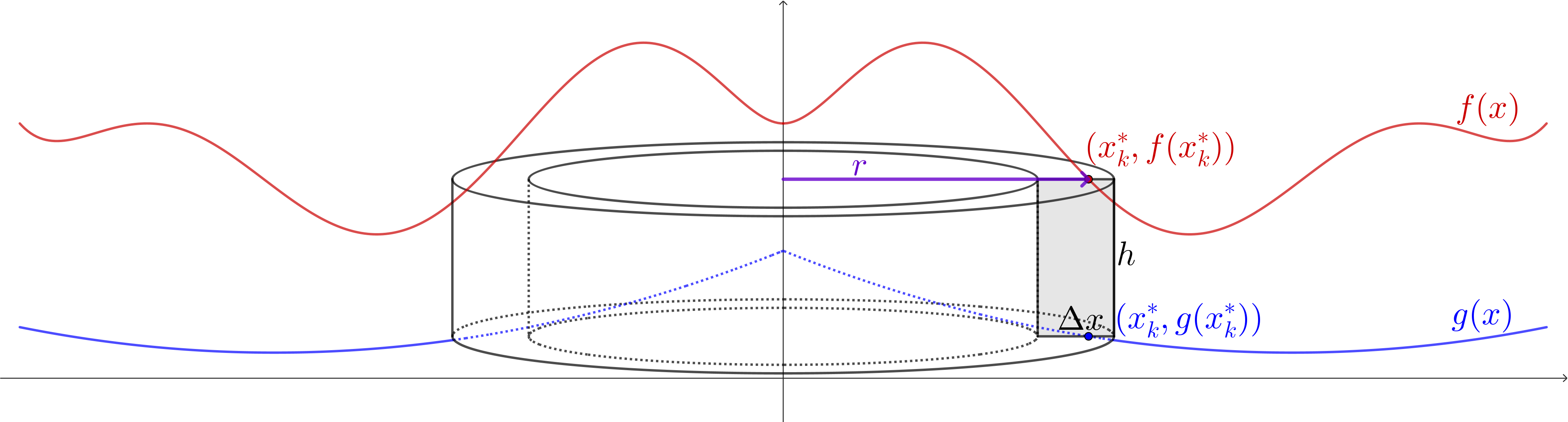
For this rectangle, we can notice that when we revolve it around the \(y\)-axis, we create a hollow cylinder. We’ll focus more specifically on this cylinder.
The single highlighted cylinder, with labels for its radius and height, as well as the thickness Delta x.
Figure 6.3.17.
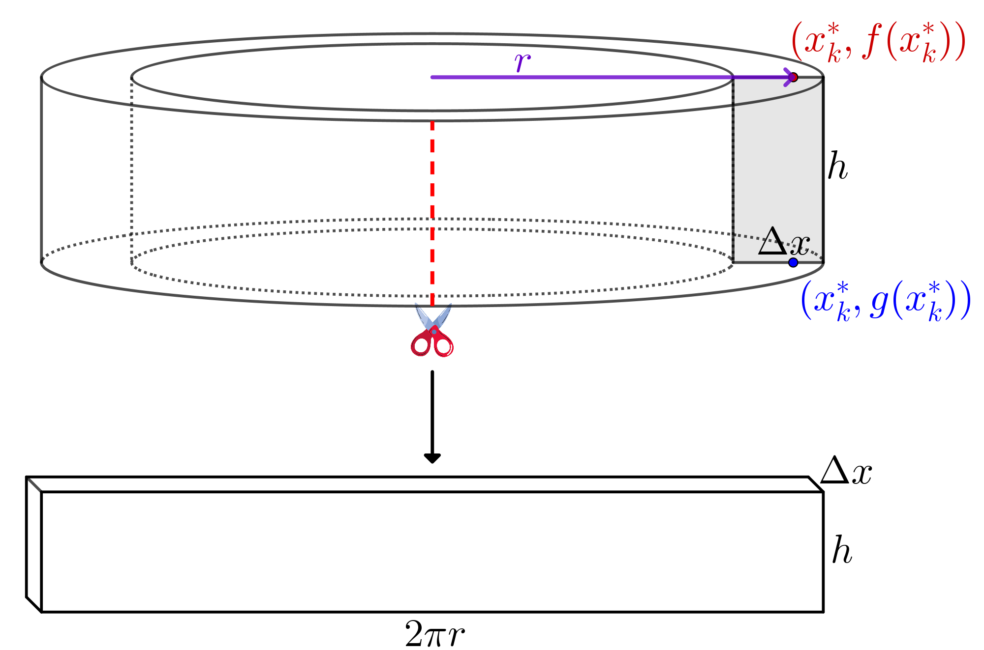
Let’s focus more on the cylinder. We’ll need to find the volume of this cylinder. We can think of this volume as really the surface area of the cylinder multiplied by the thickness. Another way to visualize it is to think about cutting the cylinder open, and unfurling it to create a rectangular solid with some thickness.
The single highlighted cylinder in isolation with a cut across it. Underneath there is an arrow pointing towards the unfurled rectangle, where the width is labeled 2*pi*r and the height is labeled h, while the thickness is Delta x.
Figure 6.3.18.
So we can see that to find \(V_k\text{,}\) we’re going to multiply \(A(x_k^*)\) and \(\Delta x\) again, where \(A(x_k^*)\) is the area of the cross-sectional "face." In this case, we can see how we’ll construct this from the unfurled cylinder.
\begin{align*} V_k \amp= 2\pi r \Delta x \\ \amp = 2\pi (x_k^*)(f(x_k^*)-g(x_k^*))\Delta x\\ V \amp \approx \sum_{k=1}^n 2\pi (x_k^*)(f(x_k^*)-g(x_k^*))\Delta x\\ V \amp = \lim_{n\to\infty} \sum_{k=1}^n 2\pi (x_k^*)(f(x_k^*)-g(x_k^*))\Delta x\\ \amp = \int_{x=a}^{x=b} 2\pi x(f(x)-g(x))\;dx \end{align*}

Definition 6.3.19. Volume by Shells.

If \(f(x)\) and \(g(x)\) are continuous functions with \(f(x)\geq g(x)\) on the interval \([a,b]\) (with \(a\geq0\)), then the volume of the solid formed when the region bounded between the curves \(y=f(x)\) and \(y=g(x)\) from \(x=a\) to \(x=b\) is revolved around the \(y\)-axis is
\begin{equation*} V = 2\pi \int_{x=a}^{x=b} x\left(f(x)-g(x)\right)\;dx\text{.} \end{equation*}
We can apply this formula in a familiar example, and also practice changing variables.

Activity 6.3.4. Volume by Shells.

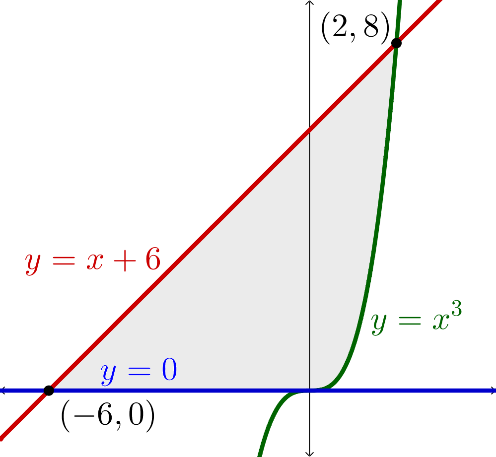
Let’s consider the region bounded by the curves \(y=x^3\) and \(y-x+6\) as well as the line \(y=0\text{.}\) You might remember this region from Activity 6.2.3. This time, we’ll create a 3-dimensional solid by revolving the region around the \(x\)-axis
A graph of the two curves y=x+6 and y=x^3 as well as the line y=0. The region trapped inside is shaded, and the intersection points (-6,0) and (2,8) are labelled.
Figure 6.3.20.
(a)
Sketch one or two rectangles that are perpendicular to the \(x\)-axis. Then set up an integral expression to find the volume of the solid using them.
Hint.
Note that in this context, we’re actually using disks and washers. Also note that the bottom of the rectangles are bounded by \(y=0\) from \(x=-6\) to \(x=0\) and then switches to being bounded by \(y=x^3\) from \(x=0\) to \(x=2\text{.}\)
Answer.
\begin{equation*} V = \pi \int_{x=-6}^{x=0}(x+6)^2\;dx + \pi \int_{x=0}^{x=2} (x+6)^2 - (x^3)^2\;dx \end{equation*}
(b)
Now, draw a single rectangle in the region that is parallel to the axis of revolution. Use this rectangle to visualize the \(k\)th slice of this 3-dimensional solid. What does that single rectangle create when it is revolved around the \(x\)-axis?
Hint.
This won’t create a disk or washer! We’ll have to change variables, and try to see how we can create a shell.
(c)
Set up the integral expression representing the volume of the solid.
Answer.
\begin{equation*} V = 2\pi \int_{y=0}^{y=8} y(\sqrt[3]{y} - (y-6))\;dy \end{equation*}
(d)
Confirm that your volumes are the same, no matter your approach to setting it up.
To finish things up, let’s look at another interactive graph (similar to how we ended Section 6.2 Area Between Curves) that can help show the differences between finding volume with regard to \(x\) (using \(\Delta x\) in our rectangles and \(dx\) in our integrals) and finding volume with regard to \(y\) (using \(\Delta y\) in our rectangles and \(dy\) in our integrals), and how this choice changes our method from washers to shells depending on the axis of revolution.

Practice Problems Practice Problems

1.

We say that the volume of a solid can be thought of as \(\displaystyle \int_{x=a}^{x=b}A(x)\;dx\) where \(A(x)\) is a function describing the cross-sectional area of our solid at an \(x\)-value between \(x=a\) and \(x=b\text{.}\) Explain how this integral formula gets built, referencing the slice-and-sum (Riemann sum) method.

2.

Explain the differences and similarities between the disk and washer methods for finding volumes of solids of revolution.

3.

When do we integrate with regard to \(x\) (using a \(dx\) in our integral and writing our functions with \(x\)-value inputs) and when do we integrate with regard to \(y\) (using a \(dy\) in our integral and writing our functions with \(y\)-value inputs) when we’re finding volumes using disks and washers? How do we know?

4.

For each of the solids described below, set up an integral using the disk/washer method that describes the volume of the solid. It will be helpful to visualize the region, a rectangle on that region, as well as the rectangle revolved around the axis of revolution.
(a)
The region bounded by the curve \(y=2x\) and the lines \(y=0\) and \(x=3\text{,}\) revolved around the \(x\)-axis.
Hint.
(b)
The region bounded by the curve \(y=e^{-2x}\) and the \(x\)-axis between \(x=0\) and \(x=\ln(2)\text{,}\) revolved around the \(x\)-axis.
Hint.
(c)
The region bounded by the curves \(y=\ln(x)\) and \(y=\sqrt{x}\) between \(y=0\) and \(y=1\text{,}\) revolved around the \(y\)-axis.
Hint.
(d)
The region bounded by the curves \(y=2x+1\) and \(y=x\) between \(x=0\) and \(x=3\text{,}\) revolved around the \(x\)-axis.
Hint.
(e)
The region bounded by the curve \(y=x^3\text{,}\) the \(x\)-axis, and the line \(x=2\text{,}\) revolved around the \(y\)-axis.
Hint.
(f)
The region bounded by the curve \(y=x^3\) and the \(y\)-axis between \(y=0\) and \(y=2\text{,}\) revolved around the \(y\)-axis.
Hint.

5.

Explain where the pieces of the shell formula come from. How is this different than using disks/washers?

6.

Say we’re revolving a region around the \(x\)-axis to create a solid. Using the disk/washer method, we will integrate with respect to \(x\text{.}\) Using the shell method, we integrate with respect to \(y\text{.}\) Explain the difference, and why this difference occurs.

7.

For each of the solids described below, set up an integral using the shell method that describes the volume of the solid. It will be helpful to visualize the region, a rectangle on that region, as well as the rectangle revolved around the axis of revolution.
(a)
The region bounded by the curve \(y=3x\) and the lines \(x=0\) and \(y=5\text{,}\) revolved around the \(y\)-axis.
Hint.
(b)
The region bounded by the curve \(y=\sqrt{x}\) and the \(x\)-axis between \(x=0\) and \(x=9\text{,}\) revolved around the \(x\)-axis.
Hint.
(c)
The region bounded by the curves \(y=2-x^2\) and \(y=x\) and the line \(x=0\) revolved around the \(y\)-axis.
Hint.
(d)
The region bounded by the curves \(y=sin(x^2)+2\) and \(y=x\) from \(x=0\) to \(x=1\text{,}\) revolved around the \(y\)-axis.
Hint.
(e)
The region bounded by the curves \(y=x^2-6x+10\) and \(y=2+4x-x^2\) revolved around the \(y\)-axis.
Hint.
(f)
The region bounded by the curves \(y=\sqrt{2x}\) and \(y=4-x\) and the \(x\)-axis between \(x=0\) and \(x=4\text{,}\) revolved around the \(x\)-axis.
Hint.

8.

Pick at least 2 integrals from Exercise 4 to rewrite using shells instead. What about those regions did you look for to choose which ones to rewrite and which ones to not?

9.

Pick at least 2 integrals from Exercise 7 to rewrite using disks/washers instead. What about those regions did you look for to choose which ones to rewrite and which ones to not?

10.

For each of the following solids, set up an integral expression using either the disk/washer method or the shell method. You don’t need to evaluate them, but you should do some careful thinking about how you set these up, especially as you choose between methods and what variable you are integrating with.
(a)
The region bounded by the curves \(y=x^2+1\) and \(y=x^3+1\) in the first quadrant, revolved around the \(x\)-axis.
Hint.
(b)
The region bounded by the curves \(y=x^2+1\) and \(y=x^3+1\) in the first quadrant, revolved around the \(y\)-axis.
Hint.
(c)
The region bounded by the curves \(y=\frac{1}{x}\) and \(y=1-(x-1)^2\) in the first quadrant, revolved around the \(x\)-axis.
Hint.