The big result from our last section on Riemann sums is not just that we can approximate areas by thinking about a bunch of small (thin) rectangles. The big result is that this strategy is scalable: we can increase \(n\text{,}\) the number of slices/rectangles, and essentially guarantee that, eventually, our approximations will be very accurate.
Now, we move from a concrete process for building rectangles to calculate areas to a more conceptual framework: what happens when \(n\to \infty\text{?}\)
SubsectionEvaluating Areas (Instead of Approximating Them)
Our goal is to move from approximating area to evaluating areas: calculating the real value of the area of these regions bounded between curves and the \(x\)-axis. We have already decided (when we built the framework for Riemann sums and made scalability and precision in our estimates a focus) that the area we’re interested in is the result of some limiting process: we increase the number of slices, \(n\text{,}\) and in turn decrease the width of each slice, \(\Delta x\text{.}\)
If \(f(x)\) is some function defined on the interval \([a,b]\) and \(\displaystyle\sum_{k=1}^n f(x_k^*)\Delta x\) is a Riemann sum with \(n\) slices and \(\Delta x = \frac{b-a}{n}\text{,}\) then we say that the definite integral of \(f(x)\) from \(x=a\) to \(x=b\) is:
\begin{equation*}
\int_{x=a}^{x=b} f(x)\;dx = \lim_{n\to\infty} \sum_{k=1}^n f(x_k^*)\Delta x
\end{equation*}
if this limit exists. When this limit exists, we say that \(f(x)\) is integrable on the interval \([a,b]\text{.}\)
We call \(x=a\) and \(x=b\) the limits of integration for this definite integral, and we read \(\displaystyle \int_{x=a}^{x=b} f(x)\;dx\) as “the integral from \(x=a\) to \(x=b\) of \(f(x)\) with regard to \(x\text{,}\)” or sometimes we might just say “of \(f(x)\;dx\)” for short.
This is assuming we’re using a Regular Partition (Note 5.2.4). If we are not, and each slice has its own width called \(\Delta x_k\text{,}\) then the definition of a definite integral requires that as \(n\to \infty\) we see \(\Delta x_k\to 0\) for all \(k=1,2,...,n\text{.}\) Essentially, we need all of the widths to eventually get tiny: we can’t let one slice take up half of the width and then let all of the other slices get tiny, since that would still be an approximation of the area we want.
We don’t need to worry about this, though, since we’ll always just choose to make all of the \(\Delta x_k\)’s the same size: \(\Delta x = \frac{b-a}{n}\text{.}\)
Let’s say we want to calculate \(\displaystyle \int_{x=0}^{x=2} (x^2+1)\;dx\text{.}\) This is the area we were estimating in Activity 5.2.2 Approximating the Area using Rectangles. How many slices did you pick at the end of this activity? How annoying was it to add up those areas?
Whatever you did, it’s not enough: even if we decided to divide this region up into \(n=1000\) pieces, this is merely an approximation of the limit we want:
There are some ways of evaluating this specific limit using some known formulas for sums of squares and end behavior limits of rational functions. But these techniques are extremely limited: we might get lucky being able to fiddle with this limit of this sum for this function, but we won’t be so lucky in general.
Instead, let’s just think about these areas, focus on what types of functions are integrable, and then build towards our end goal of connecting these areas to antiderivatives.
We’re going to now deal with the consequences of our decisions. A truth about mathematics, sometimes not an obvious truth, is that every time we state a definition, what we are actually doing is making a decision. We are deciding on some common way of classifying and describing an object. These classifications and descriptions are choices that we are making: choices to prioritize some property or aspect over a different one, choices to include or exclude a type of object into the group of things we’re interested in, and choices that come with downstream effects.
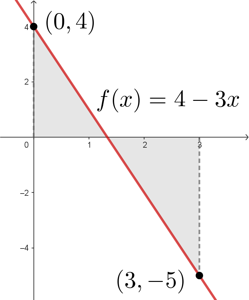
Let’s think about a simple linear function, \(f(x)=4-3x\text{.}\) We’ll both approximate and evaluate the area bounded between \(f(x)\) and the \(x\)-axis from \(x=0\) to \(x=3\text{:}\)
Explain why we do not need to think about Riemann sums in order for us to calculate the shaded area. How would you calculate this without using calculus?
You’re going to divide up the interval from \(x=0\) to \(x=3\) into 3 subintervals: \([0,1]\text{,}\)\([1,2]\text{,}\) and \([2,3]\text{.}\) Note that \(\Delta x=1\text{.}\)
Then you’re picking the left-most \(x\)-value from each subinterval (\(x_1^* = 0\text{,}\)\(x_2^* = 1\text{,}\) and \(x_3^*=2\)) to plug into \(f(x)\) in order to find the heights of your rectangles.
Let’s approximate this area a second time, but with a different selection strategy for our \(x\)-values. Calculate \(R_3\text{,}\) the Right Riemann sum with \(n=3\) rectangles.
You’re still going to divide up the interval from \(x=0\) to \(x=3\) into 3 subintervals: \([0,1]\text{,}\)\([1,2]\text{,}\) and \([2,3]\text{.}\) We still have \(\Delta x=1\text{.}\)
Then you’re picking the right-most \(x\)-value from each subinterval (\(x_1^* = 1\text{,}\)\(x_2^* = 2\text{,}\) and \(x_3^*=3\)) to plug into \(f(x)\) in order to find the heights of your rectangles.
Compare your answers for \(L_3\) and \(R_3\text{.}\) They should be very different. Why? What is happening that makes \(R_3\) specifically such a weird value?
Do you need to go back and recalculate the area geometrically (from the first part of this activity)? Explain why your answer for \(\displaystyle \int_{x=0}^{x=3}(4-3x)\;dx\)should be negative, based on the Riemann sums we calculated.
Depending on what you did earlier, you might have to find some ending \(x\)-value that “balances” the area above and below the \(x\)-axis. If you already did this, then you might have to find an ending \(x\)-value that collapses this shape down to a 1-dimensional shape with no area.
Weird areas, right? Negative? That’s not how we normally think about areas. So we have to be slightly careful with how we describe this new object, the definite integral, that we’ve built. We don’t need to go back and change anything about the object itself: we just need to change how we talk about it.
It’s common to think about \(\displaystyle \int_{x=a}^{x=b}f(x)\;dx\) as the “area under the curve \(f(x)\) from \(x=a\) to \(x=b\text{,}\)” but we know that’s not really true. Instead, we’ll think about it as a signed area of the region bounded between the curve \(f(x)\) and the \(x\)-axis from \(x=a\) to \(x=b\text{.}\) When we say “signed area,” we’re just referring to the consequence of using \(y\)-values to define “heights” of the rectangles: when the curve is under the \(x\)-axis, we end up with negative values for heights, and so those rectangles have negative area.
Let’s think about the same linear function, \(f(x)=4-3x\text{,}\) but this time we’ll approximate and evaluate the area bounded between \(f(x)\) and the \(x\)-axis from \(x=3\) to \(x=0\text{:}\)
Then you’re picking the middle \(x\)-value from each subinterval (\(x_1^* = \frac{1}{2}\text{,}\)\(x_2^* = \frac{3}{2}\text{,}\) and \(x_3^*={5}{2}\)) to plug into \(f(x)\) in order to find the heights of your rectangles.
Do you need to go back and recalculate the area geometrically (from the first part of this activity)? Explain why your answer for \(\displaystyle \int_{x=3}^{x=0}(4-3x)\;dx\)should be positive, based on the Riemann sums we calculated.
Ok, so we have some intuition about how the signs of these areas work, and we’ve also built up some nice properties that we can talk through. Let’s finish this section by just summarizing some of the things we’ve done and thinking about what kinds of functions this works for!
If \(f(x)\) is continuous on the interval \([a,b]\text{,}\) then \(f(x)\) is integrable on \([a,b]\text{.}\) That is, the limit \(\displaystyle \lim_{n\to\infty} \sum_{k=1}^n f(x_k^*)\Delta x\) exists and so we can evaluate the definite integral:
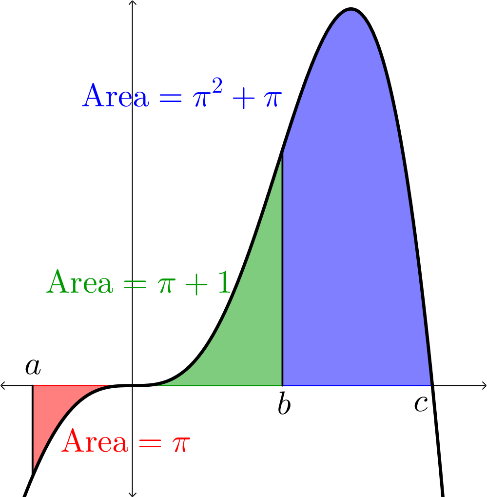
If \(a\text{,}\)\(b\text{,}\) and \(c\) are real numbers and \(f(x)\) is a function that is continuous on the intervals \([a,b]\) and \([b,c]\text{,}\) then:
Ok, that’s enough of this: let’s get to the point and try to figure out how to actually calculate these areas without relying on our functions being “nice” enough that we can use geometry!
Sketch the integral \(\displaystyle\int_{x=0}^{x=2\pi} \left(\sin(x)\right)\;dx\text{.}\) Estimate this value from the sketch you drew. Explain your answer.
For each of the following definite integrals, sketch the integral and use geometry to evaluate the definite integral. Feel free to use desmos to visualize the graphs of functions.
Say we are given that \(\displaystyle\int_{x=0}^{x=5} f(x)\;dx = 10\text{,}\)\(\displaystyle\int_{x=5}^{x=9} f(x)\;dx = -2\text{,}\) and \(\displaystyle\int_{x=0}^{x=9} g(x) \;dx = -6\text{.}\) Evaluate each of the following.