
Section 1.1 The Definition of the Limit

We’re going to start this textbook by stating a definition. This is a common practice in math classes: we need to agree upon a common definition of the mathematical objects and adjectives we are thinking about. We will state a lot of definitions in this textbook.
What I hope we will do, though, is motivate these definitions. We want to arrive at a point where it makes sense to give a name to this phenomena or object that we’re thinking of. Or maybe we arrive at a point where the specifics of the definition don’t just come down to us out of nowhere, but feel like reasonable and obvious things to consider.
So for now, we’re going to work on defining a very important and very key mathematical object that is used in calculus: the limit.
A limit is all about closeness, so let’s first interact with the idea of closeness, and then work on a definition of a limit.

Subsection Defining a Limit

Activity 1.1.1. Close or Not?

We’re going to try to think how we might define “close”-ness as a property, but, more importantly, we’re going to try to realize the struggle of creating definitions in a mathematical context. We want our definition to be meaningful, precise, and useful, and those are hard goals to reach! Coming to some agreement on this is a particularly tricky task.
(a)
For each of the following pairs of things, decide on which pairs you would classify as “close” to each other.
  • You, right now, and the nearest city with a population of 1 million or higher
  • Your two nostrils
  • You and the door of the room you are in
  • You and the person nearest you
  • The floor of the room you are in and the ceiling of the room you are in
(b)
For your classification of “close,” what does “close” mean? Finish the sentence: A pair of objects are close to each other if...
(c)
Let’s think about how close two things would have to be in order to satisfy everyone’s definition of “close.” Pick two objects that you think everyone would agree are “close,” if by “everyone” we meant:
  • All of the people in the building you are in right now.
  • All of the people in the city that you are in right now.
  • All of the people in the country that you are in right now.
  • Everyone, everywhere, all at once.
(d)
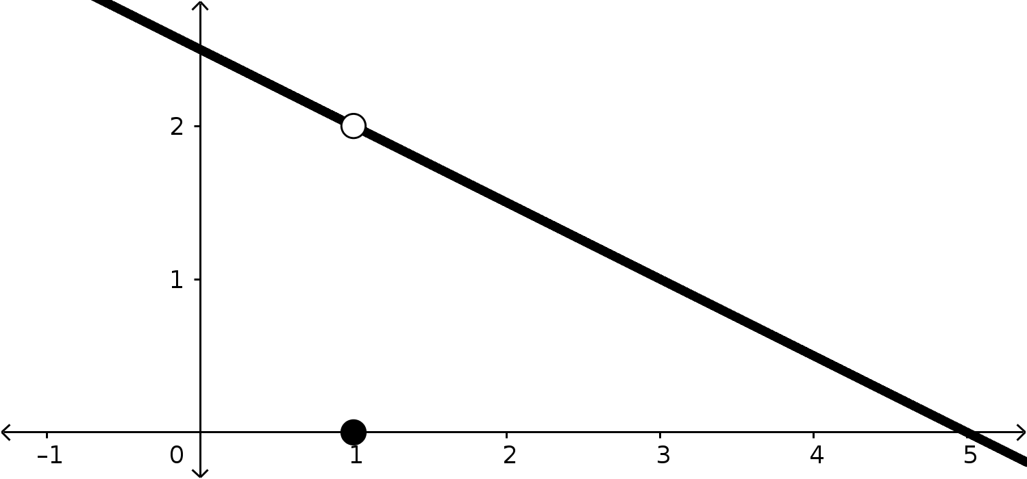
Let’s put ourselves into the context of functions and numbers. Consider the linear function \(y=4x-1\text{.}\) Our goal is to find some \(x\)-values that, when we put them into our function, give us \(y\)-value outputs that are “close” to the number 2. You get to define what close means.
First, evaluate \(f(0)\) and \(f(1)\text{.}\) Are these \(y\)-values “close” to 2, in your definition of “close?”
(e)
Pick five more, different, numbers that are “close” to 2 in your definition of “close.” For each one, find the \(x\)-values that give you those \(y\)-values.
(f)
How far away from \(x=\frac{3}{4}\) can you go and still have \(y\)-value outputs that are “close” to 2?
To wrap this up, think about your points that you have: you have a list of \(x\)-coordinates that are clustered around \(x=\frac{3}{4}\) where, when you evaluate \(y=4x-1\) at those \(x\)-values, you get \(y\)-values that are “close” to 2. Great!
Do you think others will agree? Or do you think that other people might look at your list of \(y\)-values and decide that some of them aren’t close to 2?
Do you think you would agree with other peoples’ lists? Or you do think that you might look at other peoples’ lists of \(y\)-values and decide that some of them aren’t close to 2?
The balance that we need to find, as we discovered in Activity 1.1.1, is about being able to leave room for those with a very strict idea of what “close” might be. We will want to think of an idea kind of like “infinite closeness,” but we’re not going to frame it this way: we’re going to think about a function’s output being so close to some specific number that literally everyone can agree. It is so close that it is within every possible definition of closeness.
The general idea is that we want to think about the behavior of a function at inputs that are near some specific input. Is there a trend with the outputs? Are they all centered around a specific value or do they differ wildly?

Definition 1.1.1. Limit of a Function.

For the function \(f(x)\) defined at all \(x\)-xalues around \(a\) (except maybe at \(x=a\) itself), we say that the limit of \(f(x)\) as \(x\) approaches \(a\) is \(L\) if \(f(x)\) is arbitrarily close to the single, real number \(L\) whenever \(x\) is sufficiently close to, but not equal to, \(a\text{.}\) We write this as:
\begin{equation*} \lim_{x\to a} f(x) = L \end{equation*}
or sometimes we write \(f(x) \to L\) when \(x\to a\text{.}\)
We can clarify a couple of things here:
  • There are two types of “close” in this definition: “arbitrarily close” and “sufficiently close.” One of these is in references to \(x\)-values being close to a number and the other is in reference to function outputs being close to a specific number.
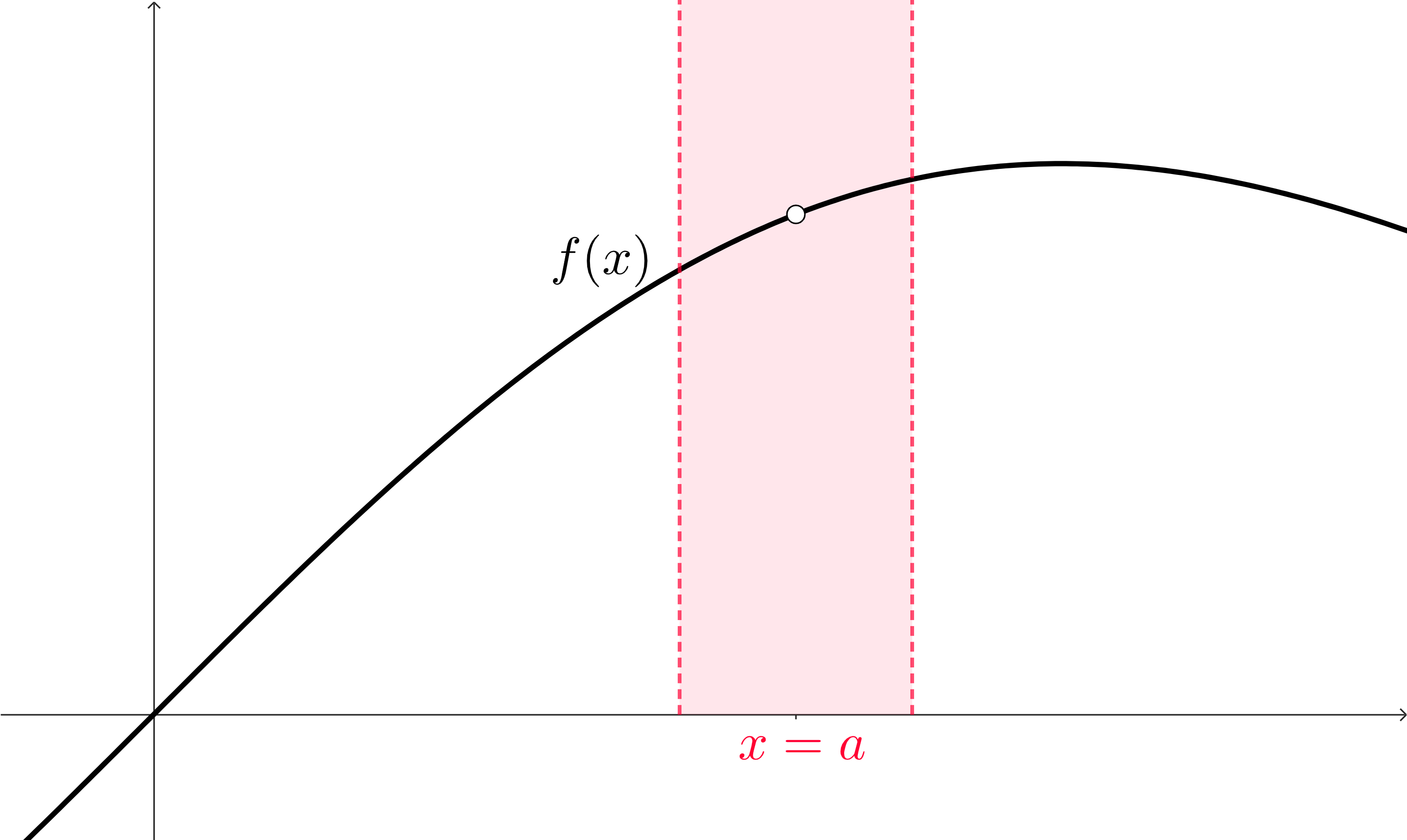
  • We are concerned with the behavior of a function around, but not at, a specific \(x\)-value: \(x=a\text{.}\) We don’t really care about what the function is doing at that input (if anything at all), and we already have words to describe that kind of behavior!
  • When we talk about \(x\)-values that are near \(a\text{,}\) that might reference \(x\)-values that are a bit bigger than \(a\) or \(x\)-values that are a bit smaller than \(a\text{.}\) We can be more specific by simply changing this definition to focus on only one “side” individually.
We can go back to Activity 1.1.1 and think about how we chose \(x\)-values that were larger than \(\frac{3}{4}\) and smaller than \(\frac{3}{4}\text{.}\) Let’s define these ideas a bit more formally!

Definition 1.1.2. Left-Sided Limit.

For the function \(f(x)\) defined at all \(x\)-xalues around and less than \(a\text{,}\) we say that the left-sided limit of \(f(x)\) as \(x\) approaches \(a\) is \(L\) if \(f(x)\) is arbitrarily close to the single, real number \(L\) whenever \(x\) is sufficiently close to, but less than, \(a\text{.}\) We write this as:
\begin{equation*} \lim_{x\to a^-} f(x) = L \end{equation*}
or sometimes we write \(f(x) \to L\) when \(x\to a^-\text{.}\)

Definition 1.1.3. Right-Sided Limit.

For the function \(f(x)\) defined at all \(x\)-xalues around and greater than \(a\text{,}\) we say that the right-sided limit of \(f(x)\) as \(x\) approaches \(a\) is \(L\) if \(f(x)\) is arbitrarily close to the single, real number \(L\) whenever \(x\) is sufficiently close to, but greater than, \(a\text{.}\) We write this as:
\begin{equation*} \lim_{x\to a^+} f(x) = L \end{equation*}
or sometimes we write \(f(x) \to L\) when \(x\to a^+\text{.}\)
This should lead us to our first result in this textbook. This first result will do two things:
  1. Introduce some language that we can use when we talk about limits as well as a classification that we can apply to them.
  2. Introduce how we will build our results throughout the course of this text. We want to discover these results as things that are required for us to talk about (and do) calculus together, and hopefully we can motivate each one beforehand.
In lieu of a formal activity, let’s just review Definition 1.1.1 Limit of a Function pose the following questions to think about:
  • Why do we put emphasis on \(L\) being a number? What could happen if it wasn’t?
  • Why do we put the emphasis on the number \(L\) being a real number? What other type(s) of number could it be?
  • Why do we put emphasis on \(L\) being a single number? How could we have the function be close to multiple real numbers?
We can look at one of the ways that we break the definition: by having two different values that the function gets close to.

Subsection Approximating Limits Using Our New Definition

We have defined a new term, and now we do the typical mathematical task: define a new thing and then investigate it.
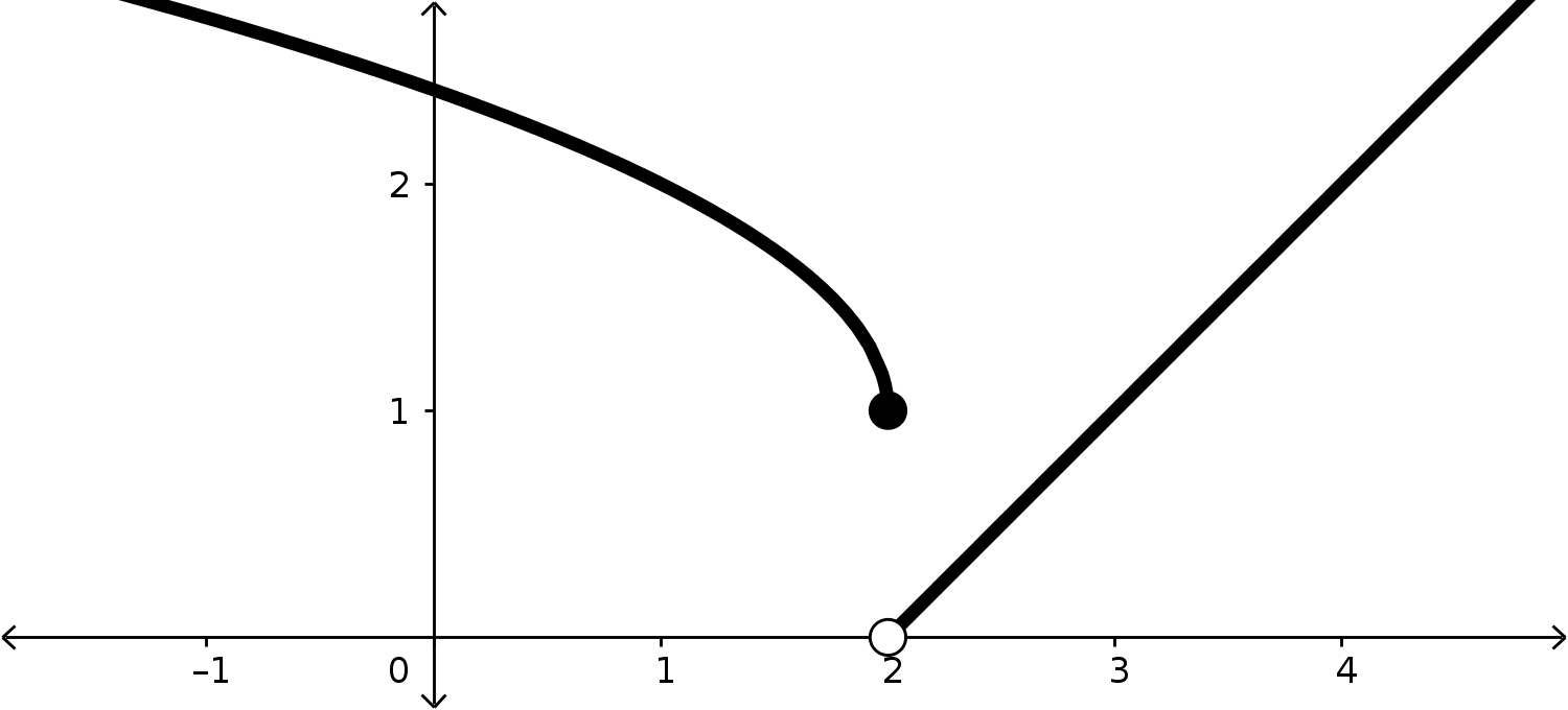
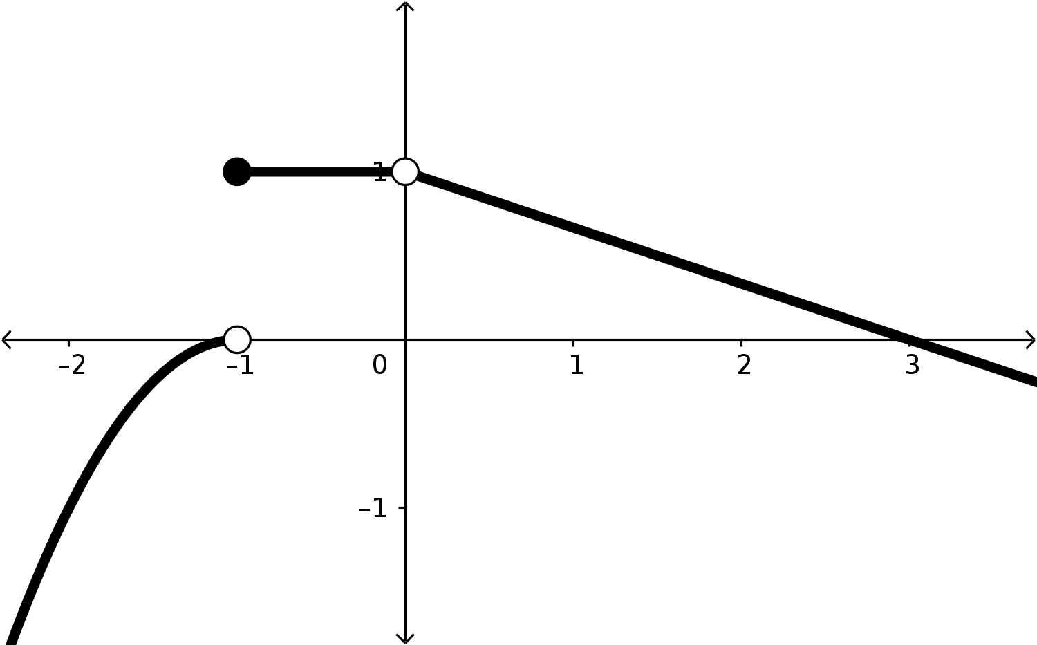
We will eventually get really good at thinking about limits and using them, but for now we just want to get familiar with them. Let’s approximate these values that our function is near by looking at some pictures of graphs and some tables of function outputs.
Later on, we’ll formalize this more. For now, we just want to use these pictures and tables to get familiar with what a limit even is.

Activity 1.1.2. Approximating Limits.

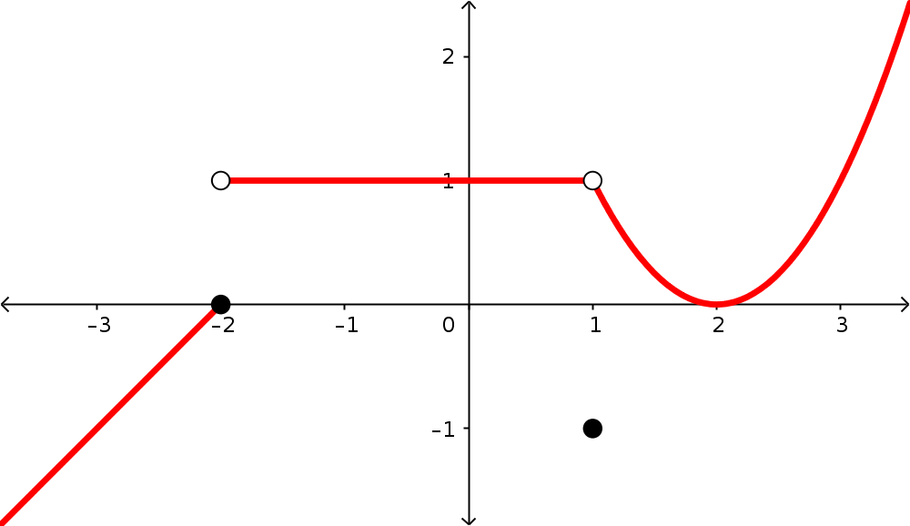
For each of the following graphs of functions, approximate the limit in question. When you do so, approximate the values of the relevant one-sided limits as well.
(a)
Approximate \(\displaystyle \lim_{x\to 1} f(x)\) using the graph of the function \(f(x)\) below.
A decreasing linear function with a single point removed from the line. At the x-value x=1, there is a hole on the line at y=1, and a point is located at (1,0).
Figure 1.1.5.
(b)
Approximate \(\displaystyle \lim_{x\to 2} g(x)\) using the graph of the function \(g(x)\) below.
A piecewise defined function, where the graph is split up into two sections around x=2. For x-values less than (and equal) to 2, the function is decreasing and curves downward towards a filled in point at (2,1). Then the graph drops to an open point at (2,0), where the graph is linear and increasing afterwards from that hole.
Figure 1.1.6.
(c)
Approximate the following three limits using the graph of the function \(h(x)\) below.
  • \(\displaystyle \displaystyle \lim_{x\to -1} h(x)\)
  • \(\displaystyle \displaystyle \lim_{x\to 0} h(x)\)
  • \(\displaystyle \displaystyle \lim_{x\to 2} h(x)\)
A piecewise-defined fucntion with three distinct pieces. For x-values less than -1, the graph is increasing and curves towards an open hole at (-1,0). Then, at x=-1, we have a point at (-1,1). The graph is constant at y=1 until a hole at (0,1). After this hole, it decreases from (0,1) towards and through (3,0) linearly.
Figure 1.1.7.
(d)
Why do we say these are “approximations” or “estimations” of the limits we’re interested in?
(e)
Are there any limit statements that you made that you are 100% confident in? Which ones?
(f)
Which limit statements are you least confident in? What about them makes them ones you aren’t confident in?
(g)
What extra details would you like to see to increase the confidence in your estimations? Are there changes we could make to the way these functions are represented that would make these approximations better or easier to make?
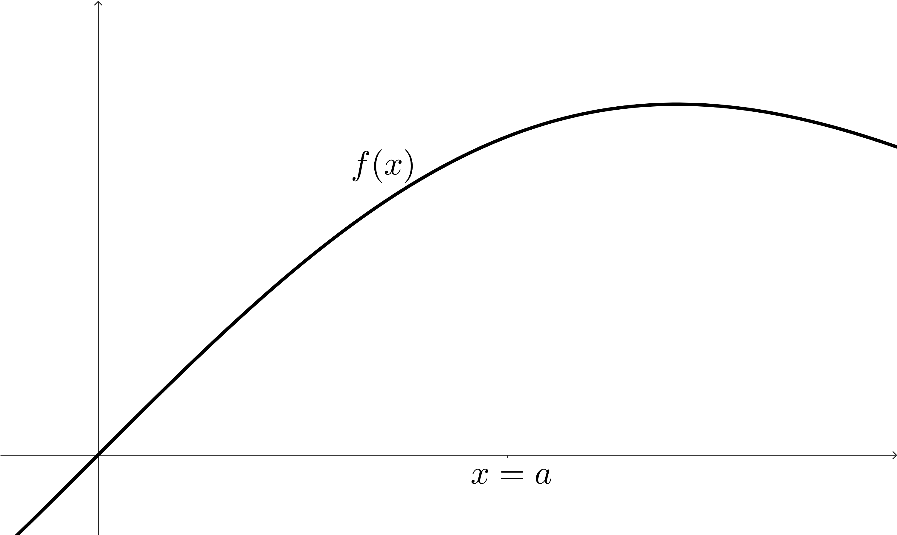
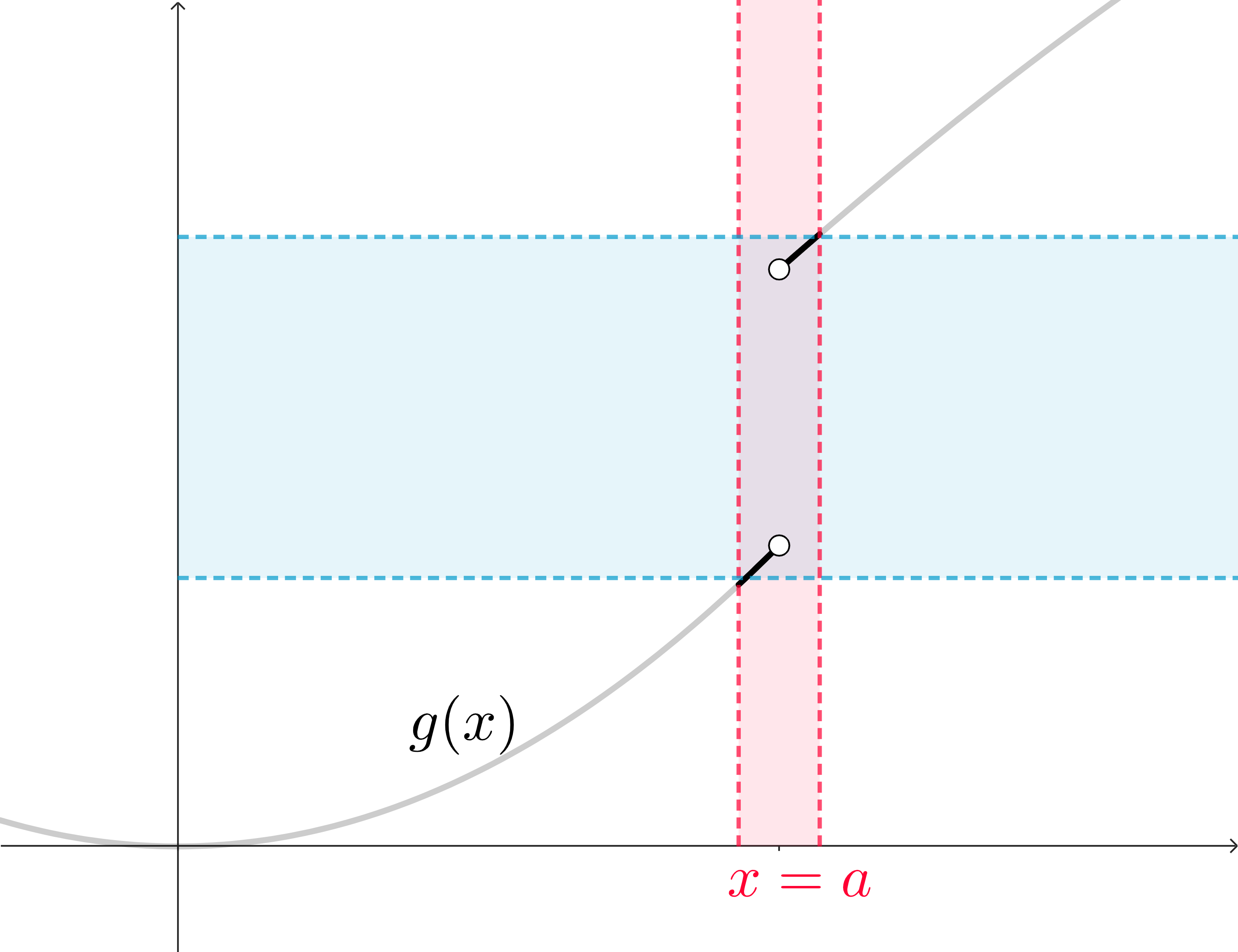
It can be hard to focus on the aspects of a graph that we really care about for the purpose of a limit. Let’s build a small strategy to help us think about what we’re looking at. We’ll start by just considering some function, \(f(x)\text{.}\) Using our definition of the Limit of a Function as a guide, we’ll make sure that it’s defined around some \(x\)-value, \(x=a\text{.}\)
The graph of a function f(x). It passes through the origin and then curves a bit in the first quadrant. There is a label for x=a on the horizontal axis.
Figure 1.1.8. The function, \(f(x)\text{.}\)
Now we want to investigate more of our definition. We want to look at the \(x\)-values that are around, but not equal to, \(x=a\text{.}\)
The graph of a function f(x). Around x=a is a vertical band, representing the interval of x-values around x=a.
Figure 1.1.9. The \(x\)-values around \(x=a\text{.}\)
The graph of a function f(x). Around x=a is a vertical band, representing the interval of x-values around x=a, and the point at x=a has been removed.
Figure 1.1.10. The \(x\)-values around, but not equal to, \(x=a\text{.}\)
We can see that we might as well remove any point at \(x=a\) from our graph: we are only concerned with the behavior around that \(x\)-value instead of the function’s behavior at it.
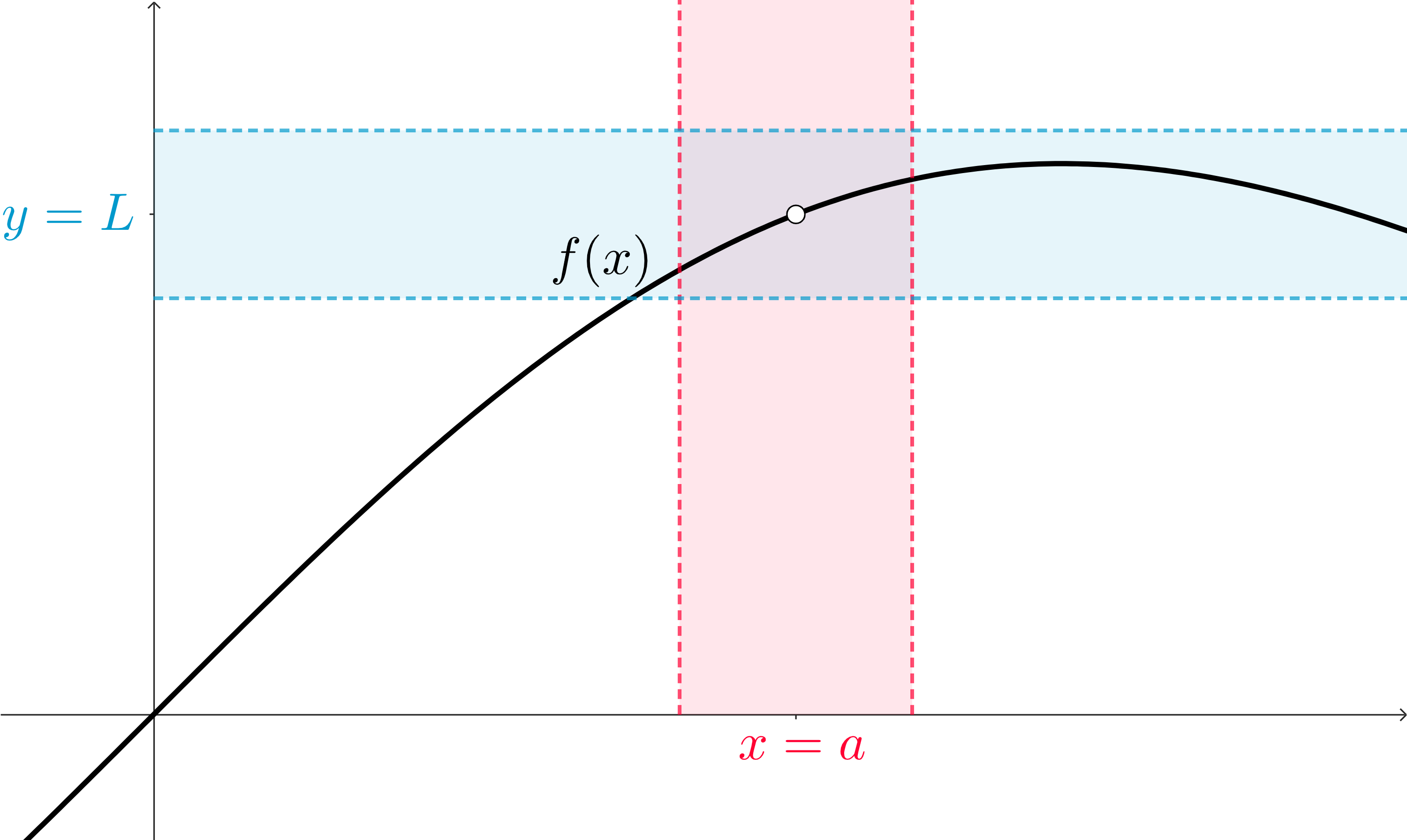
And now our focus can turn to the function outputs. For the \(x\)-values in this interval of inputs that we’ve constructed, is there some common real number that the corresponding function outputs are close to? We can visualize some interval of \(y\)-values. We’ll think of this as a target: we want to build an interval of \(y\)-values that all of the function outputs from this interval of \(x\)-values land in.
The graph of a function f(x). Around x=a is a vertical band, representing the interval of x-values around x=a, and there is a corresponding horizontal band of y-values surrounding a label y=L.
Figure 1.1.11. The corresponding function outputs \(f(x)\) are all in the target interval of \(y\)-values.
This is a pretty wide range of \(y\)-values, but we can see that the graph of the function (when we limit to just the interval of \(x\)-values selected) produces function outputs that exist only in that interval. We don’t fill the interval, but that’s fine!
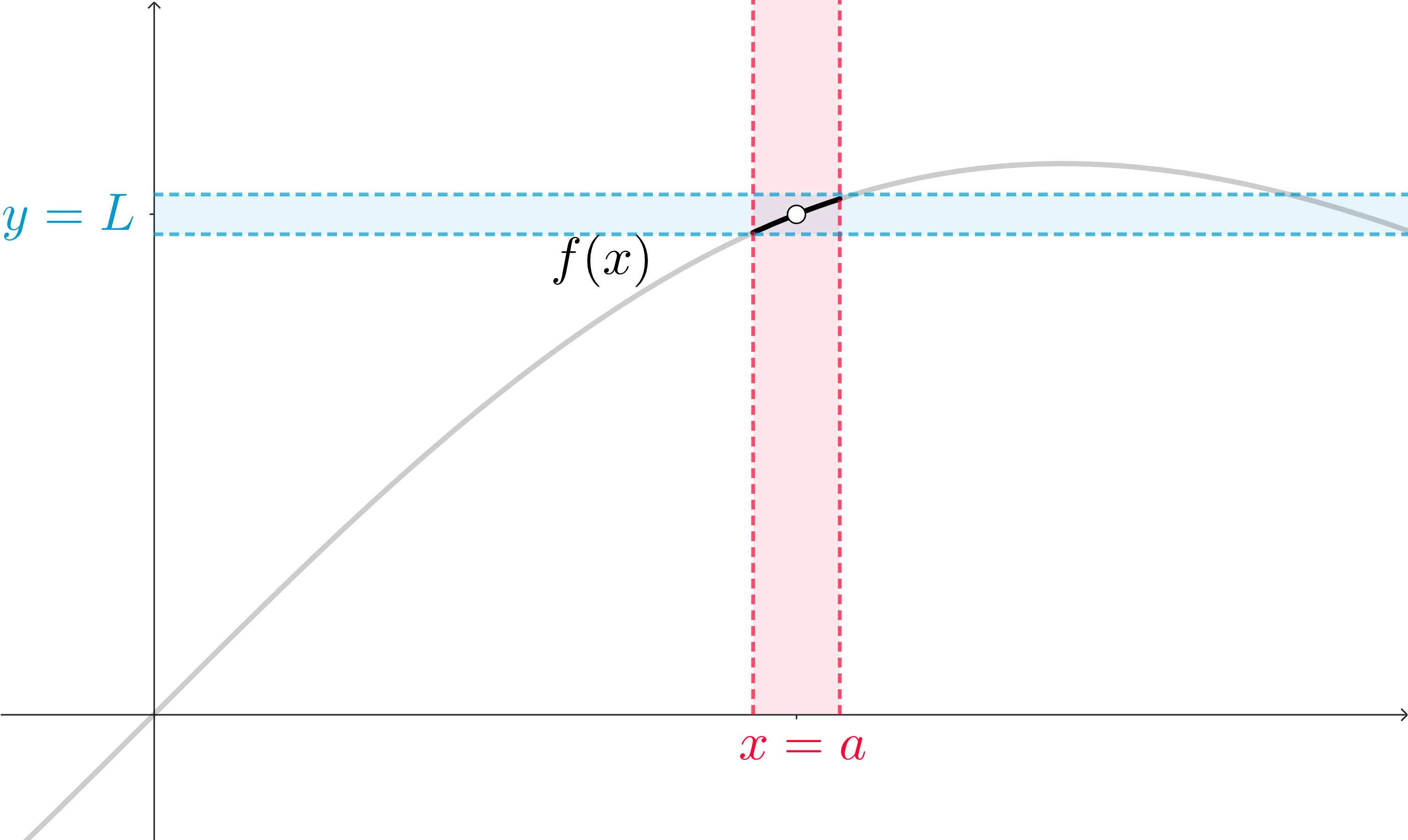
What we really care about, though, is if these function outputs are all close to the same, single, real number. What we can do is look at a more strict idea of “closeness” in the \(y\)-interval by shrinking it. In order for us to produce function outputs that are in this new, smaller, interval, we’ll need to correspondingly shrink our interval of inputs to more closely surround \(x=a\text{.}\)
The graph of a function f(x) is highlighted in the interval of x-values. The interval of y-values is smaller, as is the interval of x-values.
Figure 1.1.12. The \(x\)-values around, but not equal to, \(x=a\text{.}\)
In this visualization, we’ve also tried to focus on just the portion of our function that exists in this little intersection of intervals: we want to know what these functions values are close to, or more specifically if they are all close to the same thing. So we can de-emphasize the rest of our function!
All we’re doing is working on a strategy to focus on the parts of this graph that matter: only the parts of the curve that are surrounding \(x=a\) (but not that actual point specifically). From there, we just want to know what the function outputs are clustered around, if anything.
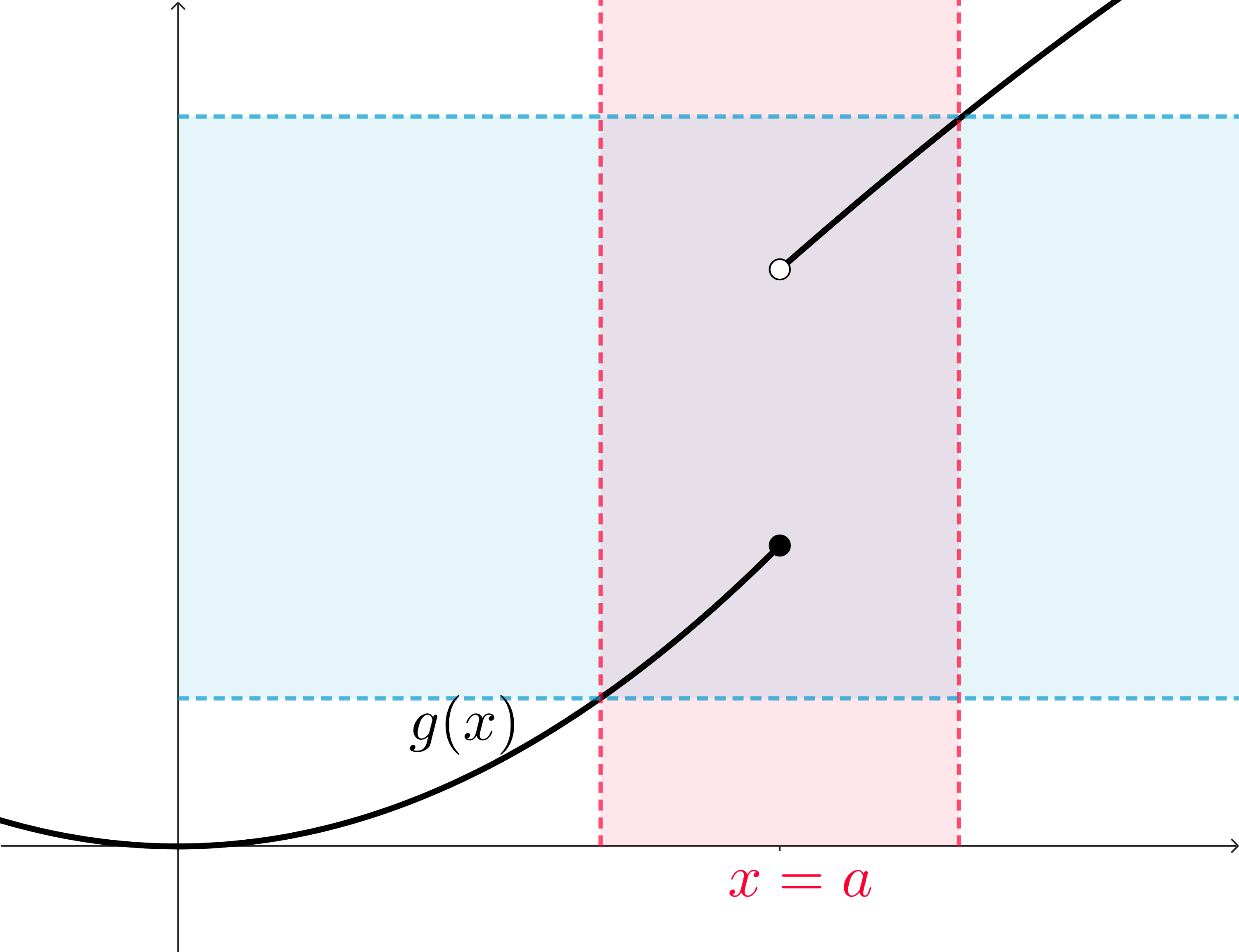
Let’s look at this same kind of visualization for a limit that does not exist: we’re going to think about the case where the one-sided limits don’t match. We’ll start a little further on in this visualization process: we have a function, and we can visualize an interval of \(x\)-values whose function outputs land inside a target interval of \(y\)-values.
The graph of a function g(x). Around x=a is a vertical band, representing the interval of x-values around x=a, and there is a corresponding horizontal band of y-values. The function itself is a piecewise function and has a big vertical gap at x=a.
Figure 1.1.13.
We can see the problem: that vertical space between the function on the left of \(x=a\) and the where the function values are on the right of \(x=a\) will make it so that horizontal bar cannot get much smaller. We can disregard the point at \(x=a\) as well as the function outside of the interval, but once try to shrink the target interval of \(y\)-values, but we’ll see the problem.
The graph of a function g(x). Around x=a is a vertical band, representing the interval of x-values around x=a, and there is a corresponding horizontal band of y-values. The function itself is a piecewise function and has a big vertical gap at x=a.
Figure 1.1.14.
These function outputs are spread apart! They are not close to a single value. Instead, they’re close to two! The function is close to a value on the left side, and then the function is close to a larger value on the right side.
\begin{equation*} \lim_{x\to a^-} g(x) \neq \lim_{x\to a^+} g(x) \text{ and so } \lim_{x\to a} g(x) \text{ does not exist}\text{.} \end{equation*}
Now let’s think about how we can approximate (and learn more about) limits using when we just think about the actual values of a function’s inputs and corresponding outputs.

Activity 1.1.3. Approximating Limits Numerically.

For each of the following tables of function values, approximate the limit in question. When you do so, approximate the values of the relevant one-sided limits as well.
(a)
Approximate \(\displaystyle \lim_{x\to 1} f(x)\) using the table of values of \(f(x)\) below.
Table 1.1.15.
\(x\) 0.5 0.9 0.99 1 1.01 1.1 1.5
\(f(x)\) 8.672 9.2 9.0001 -7 8.9998 9.5 7.59
(b)
Approximate \(\displaystyle \lim_{x\to -3} g(x)\) using the table of values of \(g(x)\) below.
Table 1.1.16.
\(x\) -3.5 -3.1 -3.01 -3 -2.99 -2.9 -2.5
\(g(x)\) -4.41 -3.89 -4.003 -4 7.035 2.06 -4.65
(c)
Approximate \(\displaystyle \lim_{x\to \pi} h(x)\) using the table of values of \(h(x)\) below.
Table 1.1.17.
\(x \) 3.1 3.14 3.141 \(\pi\) 3.142 3.15 3.2
\(h(x)\) 6 6 6 undefined 5.915 6.75 8.12
(d)
Are you 100% confident about the existence (or lack of existence) of any of these limits?
(e)
What extra details would you like to see to increase the confidence in your estimations? Are there changes we could make to the way these functions are represented that would make these approximations better or easier to make?
Overall, there’s a common theme here: in either representation (graphically or numerically), we’re making a best guess at the behavior of the function values around a point. We have limited information in these estimations, and so we’re doing the best we can: in graphs, we’re trying our best to make sense of the lack of precision in in the scales of our visual, and in the numerical tables we are only given a limited number of points to think about. In both cases, we are hoping to see more information to add more confidence to these estimations.
We want to make the jump from estimating these limits to evaluating them, and for that to happen, we’ll need to add more information and more precision about the behavior of our function.

Practice Problems Practice Problems

1.

Explain in your own words the meaning of:
\begin{equation*} \lim_{x\to a^-}f(x)=L\text{.} \end{equation*}

2.

Explain in your own words the meaning of:
\begin{equation*} \lim_{x\to a^+}f(x)=L\text{.} \end{equation*}

3.

Explain in your own words the meaning of:
\begin{equation*} \lim_{x\to a}f(x)=L\text{.} \end{equation*}

4.

Say we know that \(\displaystyle\lim_{x\to3^-} f(x)=2\) and \(\displaystyle\lim_{x\to 3^+}f(x)=2\text{.}\) What do we know (specifically or in general, if anything) about each of the following?
(a)
\(f(3)\)
Solution.
We do not know anything about the value of \(f(3)\text{,}\) including whether or not there is such a value.
(b)
\(f(2.999)\)
Solution.
The value of \(f(2.999)\) should be close to the number \(2\text{.}\) We do not know exactly what the value is, though.
(c)
\(f(3.001)\)
Solution.
The value of \(f(3.001)\) should be close to the number \(2\text{.}\) We do not know exactly what the value is, though.
(d)
\(\displaystyle\lim_{x\to 3}f(x)\)
Solution.
Since both the left and the right sided limits are the same single, real number (2), so is the limit: \(\displaystyle\lim_{x\to 3}f(x)=2\text{.}\)

5.

Which of the following is possible? Explain why or why not, and any other conclusions that we can draw.
(a)
For some function \(f(x)\text{,}\) \(\displaystyle\lim_{x\to 5} f(x)=6\) and \(f(5)=-3\)
Solution.
This is possible.
(b)
For some function \(g(x)\text{,}\) \(\displaystyle\lim_{x\to 4^-} g(x) = -\dfrac{3}{2}\) and \(\displaystyle\lim_{x\to 4^+}g(x) = \dfrac{4}{7}\text{.}\)
Solution.
This is possible, although it means that \(\displaystyle\lim_{x\to 4}g(x)\) does not exist.
(c)
For some function \(\ell(t)\text{,}\) \(\displaystyle \lim_{t\to \alpha} \ell(t) = 2\) and \(\displaystyle \lim_{t\to\alpha^+} \ell(t) = 1\text{.}\)
Solution.
This is not possible, since for \(\displaystyle \lim_{t\to\alpha} \ell(t) = 2\) we would need \(\displaystyle \lim_{t\to \alpha^+} \ell(t) = 2\) and \(\displaystyle \lim_{t\to \alpha^-} \ell(t) = 2\text{.}\)
(d)
For some function \(r(\theta)\text{,}\) \(\displaystyle\lim_{\theta\to 0}r(\theta)\) does not exist, \(\displaystyle\lim_{\theta\to 0^-}r(\theta)=\pi\text{,}\) and \(\displaystyle\lim_{\theta\to 0^+}r(\theta)=-\frac{\pi}{2}\text{.}\)
Solution.
This is possible.
(e)
For some function \(j(w)\text{,}\) \(j(4) = \pi\) while \(\displaystyle \lim_{w\to 4}j(w)\) does not exist.
Solution.
This is possible.

6.

Fill in the following tables in order to satisfy the requirements listed. Afterwards, include a sentence or two justifying your choices.
(a)
Requirements: \(\displaystyle\lim_{x\to1} f(x)=3\)
\(x\) \(0.93\) \(1\) \(1.04\)
\(f(x)\)
(b)
Requirements: \(\displaystyle\lim_{x\to-5^-} f(x)=2\text{,}\) \(f(-5)=6\text{,}\) and \(\displaystyle\lim_{x\to -5}f(x)\) doesn’t exist.
\(x\) \(-5.2\) \(-5\) \(4.98\)
\(f(x)\)
(c)
Requirements: \(f(7)\) does not exist and \(\displaystyle \lim_{x\to 7} f(x)=3\)
\(x\) \(6.985\) \(7\) \(7.002\)
\(f(x)\)
(d)
Requirements: \(\displaystyle\lim_{x\to 0^-} f(x)=\pi\) and \(\displaystyle\lim_{x\to 0^+} f(x)=e\text{.}\)
\(x\) \(-0.14\) \(0\) \(0.5\)
\(f(x)\)

7.

From the following tables, estimate/report each of the requested values. Explain your choices.
(a)
Requested: \(\displaystyle\lim_{x\to 1^-}f(x)\text{,}\) \(\displaystyle\lim_{x\to 1^+}f(x)\text{,}\) \(\displaystyle\lim_{x\to 1}f(x)\text{,}\) and \(f(1)\)
\(x\) \(0.9\) \(0.99\) \(0.999\) \(1\) \(1.001\) \(1.01\) \(1.1\)
\(f(x)\) \(2.4\) \(2.48\) \(2.4998\) \(9\) \(2.5004\) \(2.52\) \(2.8\)
Solution.
Estimated:
  • \(\displaystyle \displaystyle \lim_{x\to1^-}f(x) = 2.5\)
  • \(\displaystyle \displaystyle \lim_{x\to1^+}f(x) = 2.5\)
  • \(\displaystyle \displaystyle \lim_{x\to1}f(x) = 2.5\)
Reported: \(f(1)=9\)
(b)
Requested: \(\displaystyle\lim_{x\to 8^-}f(x)\text{,}\) \(\displaystyle\lim_{x\to 8^+}f(x)\text{,}\) \(\displaystyle\lim_{x\to 8}f(x)\text{,}\) and \(f(8)\)
\(x\) \(7.9\) \(7.99\) \(7.999\) \(8\) \(7.001\) \(7.01\) \(7.1\)
\(f(x)\) \(-1.5\) \(-1.9\) \(-1.999\) \(-2\) \(7.0001\) \(7.2\) \(7.5\)
Solution.
Estimated:
  • \(\displaystyle \displaystyle \lim_{x\to8^-}f(x) = -2\)
  • \(\displaystyle \displaystyle \lim_{x\to8^+}f(x) = 7\)
  • \(\displaystyle \lim_{x\to8}f(x)\) doesn’t exist
Reported: \(f(8)=-2\)
(c)
Requested: \(\displaystyle\lim_{x\to \pi^-}f(x)\text{,}\) \(\displaystyle\lim_{x\to \pi^+}f(x)\text{,}\) \(\displaystyle\lim_{x\to \pi}f(x)\text{,}\) and \(f(\pi)\)
\(x\) \(3.1\) \(3.14\) \(3.141\) \(\pi\) \(3.142\) \(3.15\) \(3.2\)
\(f(x)\) \(-3\) \(-3\) \(-3\) does not exist \(-3\) \(-3\) \(-3\)
Solution.
Estimated:
  • \(\displaystyle \displaystyle \lim_{x\to\pi^-}f(x) = -3\)
  • \(\displaystyle \displaystyle \lim_{x\to\pi^+}f(x) = -3\)
  • \(\displaystyle \displaystyle \lim_{x\to\pi}f(x) = -3\)
Reported: \(f(\pi)\) does not exist

8.

For each of the listed requirements, sketch a graph of a function that satisfies each. Afterwards, include a sentence or two justifying you sketch.
(a)
Requirements: \(f(6)=0\text{,}\) \(\displaystyle\lim_{x\to6 } f(x)=-2\text{,}\) \(\displaystyle\lim_{x\to-2^-}f(x)=1\text{,}\) and \(\displaystyle\lim_{x\to -2} f(x)\) does not exist.
(b)
Requirements: \(\displaystyle\lim_{\omega\to 0 } \rho(\omega)=8\text{,}\) \(\displaystyle\lim_{\omega\to2 }\rho(\omega)=-2\text{,}\) and \(\rho(2)\) does not exist.
(c)
Requirements: \(\displaystyle\lim_{t\to -3^-} q(t)=0\text{,}\) \(\displaystyle\lim_{t\to-3^+} q(t)=4\text{,}\) \(\displaystyle\lim_{t\to -1} q(t)=9\text{,}\) and \(q(-1)=9\text{.}\)

9.

From the graph of \(f(x)\) below, estimate of each of the requested values. Explain each of your choices.
A piecwise defined function. It is linear, traveling upwards towards a closed point at (-2,0). Then, at an open point at (-2,1), it is constant until an open point at (1,1). There is a closed point at (1,-1). The function continues at the open point at (1,1) in a parabolic shape, decreasing towards (2,0) where it turns and increases.
Figure 1.1.18. The function \(f(x)\text{.}\)
(a)
\(\displaystyle\lim_{x\to-2^-}f(x)\)
Solution.
\(\displaystyle\lim_{x\to-2^-}f(x)=0\)
(b)
\(\displaystyle\lim_{x\to-2^+}f(x)\)
Solution.
\(\displaystyle\lim_{x\to-2^+}f(x)=1\)
(c)
\(\displaystyle\lim_{x\to-2}f(x)\)
Solution.
\(\displaystyle\lim_{x\to-2}f(x)\) doesn’t exist, since the left and right sided limits don’t match.
(d)
\(\displaystyle\lim_{x\to 0^-}f(x)\)
Solution.
\(\displaystyle\lim_{x\to 0^-}f(x)=1\)
(e)
\(\displaystyle\lim_{x\to 0^+}f(x)\)
Solution.
\(\displaystyle\lim_{x\to 0^+}f(x)=1\)
(f)
\(\displaystyle\lim_{x\to 0}f(x)\)
Solution.
\(\displaystyle\lim_{x\to 0}f(x)=1\)
(g)
\(\displaystyle\lim_{x\to 1^-}f(x)\)
Solution.
\(\displaystyle\lim_{x\to 1^-}f(x)=1\)
(h)
\(\displaystyle\lim_{x\to 1^+}f(x)\)
Solution.
\(\displaystyle\lim_{x\to 1^+}f(x)=1\)
(i)
\(\displaystyle\lim_{x\to 1}f(x)\)
Solution.
\(\displaystyle\lim_{x\to 1}f(x)=1\)
(j)
\(\displaystyle\lim_{x\to 2^-}f(x)\)
Solution.
\(\displaystyle\lim_{x\to 2^-}f(x)=0\)
(k)
\(\displaystyle\lim_{x\to 2^+}f(x)\)
Solution.
\(\displaystyle\lim_{x\to 2^+}f(x)=0\)
(l)
\(\displaystyle\lim_{x\to 2}f(x)\)
Solution.
\(\displaystyle\lim_{x\to 2}f(x)=0\)