Section 10.3 Calculus with Parametric Curves

Now that we’re a bit more familiar with parametric curves, we’ll think about them in the context of calculus. There are only a few results that we’ll build, but all of them should end up being relatively intuitive, as long as we refer back to the results in our standard context.
But first, let’s introduce a really nice parametric curve that we’ll use to think about the calculus results.

Subsection The Cycloid

The cycloid is a great example of a parametric curve, because the description of the curve leads to the parametric definition of the curve.
If we paint a dot on the edge of a wheel and roll the wheel in a straight path, what path will the point trace?
The visual above is helpful in building the parametric definition of the cycloid. We start with a circle. Due to clockwise rotation (instead of the typical counter-clockwise rotation) as well as the point beginning at the bottom of the circle, we parameterize it as:
\begin{align*} x \amp = -\sin(t)\\ y \amp = -\cos(t) \end{align*}
In order to shift the circle up to be centered at \((0,1)\text{,}\) we can add \(1\) to the \(y\)-value and use the parametric curve:
\begin{align*} x \amp = -\sin(t)\\ y \amp = 1-\cos(t) \end{align*}
Then, in order to shift the circle to the right as the time changes, we add \(t\) to the \(x\)-value:
\begin{align*} x \amp = t-\sin(t)\\ y \amp = 1-\cos(t) \end{align*}
If we want to scale the circle to have a generic radius, \(r\text{,}\) we can scale the whole thing!

Definition 10.3.1 The Cycloid.

The cycloid passing through the origin and generated by a circle of radius \(r\) rolling along the \(x\)-axis from left to right is parameterized as:
\begin{align*} x \amp = r(t-\sin(t))\\ y \amp = r(1-\cos(t)) \end{align*}

Subsection Slopes of Tangent Lines

Before we begin, let’s remind ourselves of a key idea when we were introducing parametric curves: Both \(x\) and \(y\) are independent functions of some third variable (or parameter), \(t\text{.}\)
In order for us think about derivatives, we should revisit The Chain Rule.
For us to find \(\Dydx\text{,}\) we can start by finding \(\dfrac{dy}{dt}\) using the Chain Rule:
\begin{equation*} \frac{dy}{dt} = \frac{dy}{dx} \cdot \frac{dx}{dt}\text{.} \end{equation*}
Now, we can solve for \(\Dydx\text{.}\)
Now, let’s revisit the cycloid!

Activity 10.3.3 Slopes on a Cycloid.

Consider the cycloid formed by a circle with radius \(r=1\text{:}\)
\begin{align*} x \amp = t-\sin(t)\\ y \amp = 1-\cos(t) \end{align*}
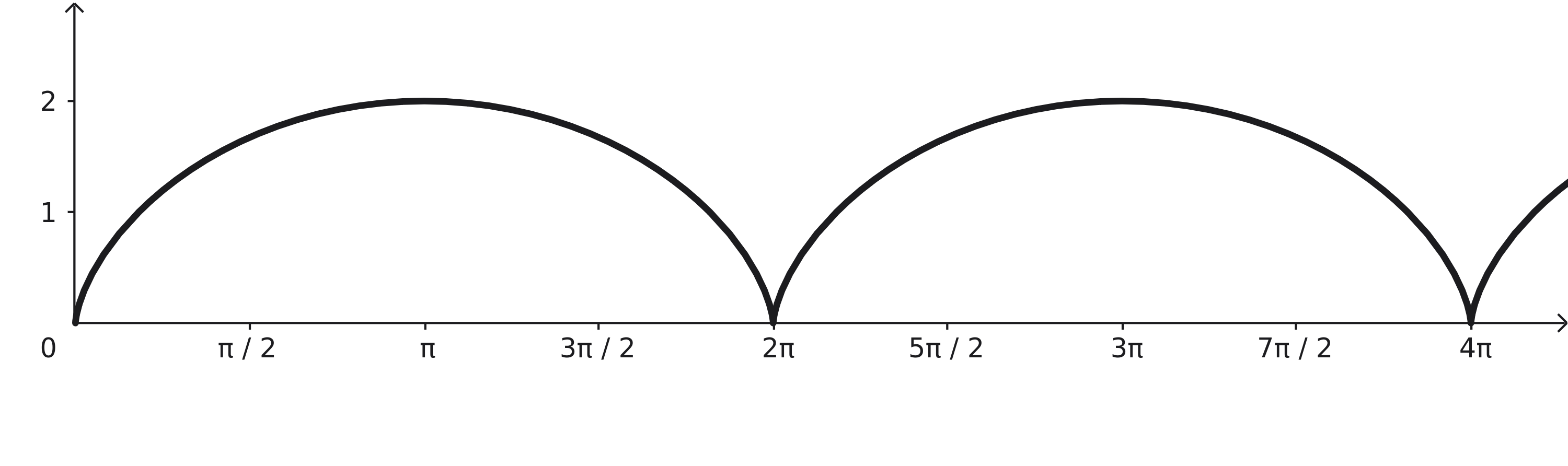
The cycloid, visualized on the interval from 0 to approximately 4 pi. This looks like 2 arches, with bottoms at 0, 2 pi and 4 pi.
Figure 10.3.4. The cycloid.

(a)

First, make a conjecture: where do you think the cycloid will have horizontal tangent lines? What about vertical tangent lines, or other points where the derivative doesn’t exist?

(b)

Find \(\frac{dy}{dt}\) and \(\frac{dx}{dt}\text{,}\) and construct \(\dydx\text{.}\)

(e)

Use these values of \(t\) to find the points on the cycloid where there are horizontal tangent lines or points where the derivative doesn’t exist. Do they match what you conjectured?

Subsection Areas Bounded by Curves

We can extend our idea from slopes, where we had to revisit the Chain Rule, towards constructing an integral for a parametric curve.
In order to find the area under a curve, we will still use the basic idea of a Riemann Sum: we want to multiply a height (\(y\)) by a width (\(dx\)) on small and specific intervals, and add them up to construct an integral.
Since our height variable, \(y\text{,}\) is a function of \(t\text{,}\) the integral will end up with an input variable that doesn’t match the differential. We can use a change of variables (like in \(u\)-Substitution) to change the differential from \(dx\) to \(dt\text{.}\)
\begin{equation*} dx = x'(t) \;dt \end{equation*}
This changes our differential, allowing us to integrate with regard to \(t\text{,}\) the input variable.

Example 10.3.6 Area Trapped in the Cycloid.

We return to the cycloid. We’ll again use the cycloid generated from a circle with radius \(r=1\text{:}\)
\begin{align*} x \amp = t-\sin(t)\\ y \amp = 1-\cos(t) \end{align*}

(a)

Set up an integral to calculate the area trapped under one arch of the cycloid.
Solution.
\begin{equation*} \int_{t=0}^{t=2\pi} \left(1-\cos(t)\right)^2\;dt \end{equation*}

(b)

Evaluate this integral!
Solution.
\begin{align*} \int_{t=0}^{t=2\pi}\left(1-\cos(t)\right)^2\;dt \amp = \int_{t=0}^{t=2\pi}\left(1 - 2\cos(t) + \cos^2(t)\right)\;dt\\ \amp = \int_{t=0}^{t=2\pi}\left(\frac{3}{2} - 2\cos(t) + \frac{1}{2}\cos(2t)\right)\;dt\\ \amp = \left(\frac{3t}{2} - 2\sin(t) - \frac{1}{4}\sin(2t)\right)\bigg|_{t=0}^{t=2\pi} \\ \amp = 3\pi \end{align*}

(c)

How does this change when the cycloid is generated from a circle with radius \(r\text{?}\)
\begin{align*} x \amp = r(t-\sin(t))\\ y \amp = r(1-\cos(t)) \end{align*}
Solution.
\begin{align*} \int_{t=0}^{t=2\pi}\left(r-r\cos(t)\right)^2\;dt \amp = r^2\int_{t=0}^{t=2\pi}\left(1-\cos(t)\right)^2\;dt\\ \amp = r^2\int_{t=0}^{t=2\pi}\left(1 - 2\cos(t) + \cos^2(t)\right)\;dt\\ \amp = r^2\int_{t=0}^{t=2\pi}\left(\frac{3}{2} - 2\cos(t) + \frac{1}{2}\cos(2t)\right)\;dt\\ \amp = r^2\left(\frac{3t}{2} - 2\sin(t) - \frac{1}{4}\sin(2t)\right)\bigg|_{t=0}^{t=2\pi} \\ \amp = 3\pi r^2 \end{align*}

Subsection Arc Lengths

We have built an arc length formula already in this textbook! Remember: DefinitionΒ 6.5.7Β Length of a Curve? Let’s rebuild this integral formula in a way that makes sense for a parametric curve.

Activity 10.3.7 Building a Parametric Arc Length Formula.

Before we begin, it might be helpful to remind yourself how we build the arclength formula in SectionΒ 6.5Β Arc Length and Surface Area.
Let’s drop back in to that derivation with some small changes. Because we’re dealing with a parametric curve, we’ll use \(t\) as our input variable, and so we’ll eventually need a \(\Delta t\) to turn into a differential \(dt\) in the integral. This means that we’ll have non-uniform \(\Delta x\) distances, since they’ll be based on the changes in the input, \(t\text{.}\) So we’ll actually use \(\Delta x_k\) to represent the change in the \(x\)-variable on the \(k\)th subinterval.
So, our length on the \(k\)th subinterval is:
\begin{equation*} \ell_k = \sqrt{(\Delta x_k)^2 + (\Delta y_k)^2} \end{equation*}

(a)

In order to build the arc length formula in SectionΒ 6.5, we factored out \(\sqrt{\Delta x^2}\) in order to end up with a \(\Delta x\) that turned into the differential \(dx\) in the integral. This time, factor out a \(\Delta t^2\) under the square root.
Solution.
\begin{align*} \ell_k \amp = \sqrt{(\Delta t)^2\left(\frac{(\Delta x_k)^2}{(\Delta t)^2} + \frac{(\Delta y_k)^2}{(\Delta t)^2}\right)}\\ \amp = \sqrt{(\Delta t)^2}\sqrt{\left(\frac{\Delta x_k}{\Delta t}\right)^2 + \left(\frac{\Delta y_k}{\Delta t}\right)^2}\\ \amp = \sqrt{\left(\frac{\Delta x_k}{\Delta t}\right)^2 + \left(\frac{\Delta y_k}{\Delta t}\right)^2} \Delta t \end{align*}

(b)

Now, create a Riemann sum and let \(n\to \infty\) (and, correspondingly, \(\Delta t\to 0\)). Note that you should end up with some differentials instead of deltas!
Solution.
\begin{align*} \ell \amp \approx \sum_{k=1}^n \sqrt{\left(\frac{\Delta x_k}{\Delta t}\right)^2 + \left(\frac{\Delta y_k}{\Delta t}\right)^2} \Delta t\\ \amp = \lim_{n\to\infty} \sum_{k=1}^n \sqrt{\left(\frac{\Delta x_k}{\Delta t}\right)^2 + \left(\frac{\Delta y_k}{\Delta t}\right)^2} \Delta t\\ \amp = \int_{t=a}^{t=b} \sqrt{\left(\frac{dx}{dt}\right)^2 + \left(\frac{dy}{dt}\right)^2}\;dt \end{align*}

Definition 10.3.8 Parametric Arc Length.

If the functions \(x(t)\) and \(y(t)\) are continuous on \([a,b]\) and differentiable on \((a,b)\text{,}\) the the length of the parametric curve
\begin{align*} x \amp = x(t)\\ y \amp = y(t) \end{align*}
on \(a\leq t\leq b\) is
\begin{equation*} \ell = \int_{t=a}^{t=b} \sqrt{(x'(t))^2+(y'(t))^2}\;dt\text{.} \end{equation*}

Example 10.3.9 Length of a Cycloid Arc.

Let’s go back, one more time, to the cycloid. We’ll again use the cycloid generated from a circle with radius \(r=1\text{:}\)
\begin{align*} x \amp = t-\sin(t)\\ y \amp = 1-\cos(t) \end{align*}

(a)

Set up the integral measuring the length of one arch of the cycloid.
Solution.
\begin{align*} \ell \amp = \int_{t=0}^{t=2\pi} \sqrt{(1-\cos(t))^2 + (\sin(t))^2}\;dt\\ \amp = \int_{t=0}^{t=2\pi} \sqrt{1-2\cos(t)+\cos^2(t) + \sin^2(t)}\;dt\\ \amp = \int_{t=0}^{t=2\pi} \sqrt{2-2\cos(t)}\;dt \\ \amp = \sqrt{2}\int_{t=0}^{t=2\pi} \sqrt{1-\cos(t)}\;dt \end{align*}

(b)

Now, evaluate the integral!
Hint.
It might help to remember a trig identity! We know \(\sin^2(\theta) = \frac{1}{2}(1-\cos(2\theta)\text{.}\) So then we can note that
\begin{equation*} \frac{1}{2}\left(1-\cos(t)\right) = \sin^2\left(\frac{t}{2}\right)\text{.} \end{equation*}
Solution.
\begin{align*} \ell \amp = \sqrt{2}\int_{t=0}^{t=2\pi} \sqrt{1-\cos(t)}\;dt\\ \amp = 2 \int_{t=0}^{t=2\pi} \sqrt{\frac{1}{2}\left(1-\cos(t)\right)}\;dt\\ \amp = 2 \int_{t=0}^{t=2\pi} \sqrt{sin^2\left(\frac{t}{2}\right)}\;dt\\ \amp = 2 \int_{t=0}^{2\pi} \sin\left(\frac{t}{2}\right)\;dt\\ \amp = 2 \left(-2\cos\left(\frac{t}{2}\right)\right)\bigg|_{t=0}^{t=2\pi}\\ \amp = 2(-2 -2)\\ \amp = 8 \end{align*}

(c)

How does this change when the cycloid is generated from a circle with radius \(r\text{?}\)
\begin{align*} x \amp = r(t-\sin(t))\\ y \amp = r(1-\cos(t)) \end{align*}
Solution.
\begin{align*} \ell \amp = \int_{t=0}^{t=2\pi} \sqrt{(r(1-\cos(t)))^2 + (r\sin(t))^2}\;dt\\ \amp = \int_{t=0}^{t=2\pi} \sqrt{r^2(1-2\cos(t)+\cos^2(t) + \sin^2(t))}\;dt\\ \amp = \int_{t=0}^{t=2\pi} r\sqrt{2-2\cos(t)}\;dt \\ \amp = r\sqrt{2}\int_{t=0}^{t=2\pi} \sqrt{1-\cos(t)}\;dt\\ \amp = 2r \int_{t=0}^{t=2\pi} \sqrt{\frac{1}{2}\left(1-\cos(t)\right)}\;dt\\ \amp = 2r \int_{t=0}^{t=2\pi} \sqrt{sin^2\left(\frac{t}{2}\right)}\;dt\\ \amp = 2r \int_{t=0}^{2\pi} \sin\left(\frac{t}{2}\right)\;dt\\ \amp = 2r \left(-2\cos\left(\frac{t}{2}\right)\right)\bigg|_{t=0}^{t=2\pi}\\ \amp = 2r(-2 -2)\\ \amp = 8r \end{align*}