It’s time for another small deviation to think about functions, again. This time, we’re going to specifically think about graphs of functions and how we visualize things.
How do we plot a typical function (in the form \(y=f(x)\)) on a coordinate grid? How do you think about the different variables, and how do we use them to plot a point?
Does the “grid” that we use match with the way you might think about locations of things in your life? Where else do humans use a grid like this to describe locations?
We’ll move forward in a familiar way. Just like in Section 10.1, we’ll ask a “What if...?” question to alter some basic ideas about how we graph things, and think about functions in a slightly different way.
What if, instead of \(x\) and \(y\) representing the horizontal and vertical locations of our point, we thought about a point’s location using a direction and a distance?
Instead of thinking about a point, \((x,y)\text{,}\) as the location described on a rectangular grid, we might think about a point described on a circular grid: the coordinates might describe a direction (an angle, measured in radians) and a distance from the origin.
This isn’t a new way of describing locations! While we might, in a city like Chicago, describe the location of something using rectangular coordinates (“My favorite sushi place is 7 blocks north and 3 block east of here.”), this isn’t the only way to describe a location. In the middle of a forest, for instance, these directions wouldn’t be helpful. Instead, we might point someone in the right direction and tell them how far away something is (“There’s a nice spot to forage for mushrooms a half a mile to the southwest of here.”).
A point \((r, \theta)\) is written in the polar coordinate system, where \(r\) represents the distance between the point and the origin (called the pole) and \(\theta\) represents the angle measured to the positive horizontal axis and a ray from the pole passing through the point.
A polar curve is a curve defined by the function \(r=f(\theta)\text{,}\) where \(\theta\) is the input/independent variable and \(r\) is the output/dependent variable.
In Step 1, explain the shape and behavior of the function based on your knowledge of trigonometric functions. How do you know, based on the function being specifically \(4\cos^2(\theta)\) that it will look like this?
In Step 2, why do the points that we filled in end up where they are on the polar curve? Explain how we use the coordinates you input in the previous step to plot these polar points.
Explain why the polar point has this shape/behavior. Refer back to explanation of the Cartesian curve in Step 1, and explain how these graphical features manifest themselves in the polar curve.
Fill in the table with the \(r\) outputs at different values of \(\theta\text{.}\) Describe why these points are plotted where they are, including the quadrants and distances from the origin/pole.
One thing to note, and focus on more closely, is our use of the word “distance” when we defined \(r\text{.}\) Our typical understanding of distance is that this is a non-negative measurement. In Activity 10.2.4 , we looked at a non-negative function, so we didn’t have to consider what might happen when our function has negative outputs. In order to give ourselves more flexibility in this coordinate system, let’s consider a new function—one with both positive and negative outputs.
In Step 1, explain how the changes to the cosine function (multiplying the input, \(\theta\) by 2 and multiplying the cosine function by 5) changes the graph from a standard cosine function’s graph. Where are the zeros, compared to where they typically are?
Fill in the table with the function outputs \(f(\theta)\) for different values of \(\theta\text{.}\) Note that the points have been colored based on the sign on the output.
Think about how \(\theta\) changes. As \(\theta\) increases, where should the points be traveling? Describe this in terms of quadrants on the graph if you’d like. Does this match the movement of the points on the polar function?
Fill in the table with the \(r\) outputs at different values of \(\theta\text{.}\) Describe why these points are plotted where they are, including the quadrants and distances from the origin/pole.
Compare the path that \(r=5\cos(2\theta)\) travels with the path that \(r=|5\cos(2\theta)|\) travels as \(\theta\) increases. What is happening to the curve when \(r=5\cos(2\theta)\) is negative?
This should be a relatively intuitive extension of our idea of “distance.” When our a polar point has a negative value of \(r\text{,}\) the point is reflected through the pole (the origin).
Before moving on, it might be nice to get more familiarity with polar plots of curves. Use the graphing utility below to look at different curves and compare the Cartesian and polar plots.
When we thought about Parametric Curves, we used a technique called Eliminating the Parameter to write a parametric curve in a more standard format, \(y=f(x)\text{.}\) It seems reasonable to come up with a way of converting a polar curve to Cartesian one, as well.
Before we tackle this, we’ll focus on converting the coordinates of a single point: we’ll see how we can write the coordinates of a polar point in the Cartesian coordinate system and the coordinates of a Cartesian point in the polar coordinate system.
Activity10.2.7Converting the Coordinates of a Point.
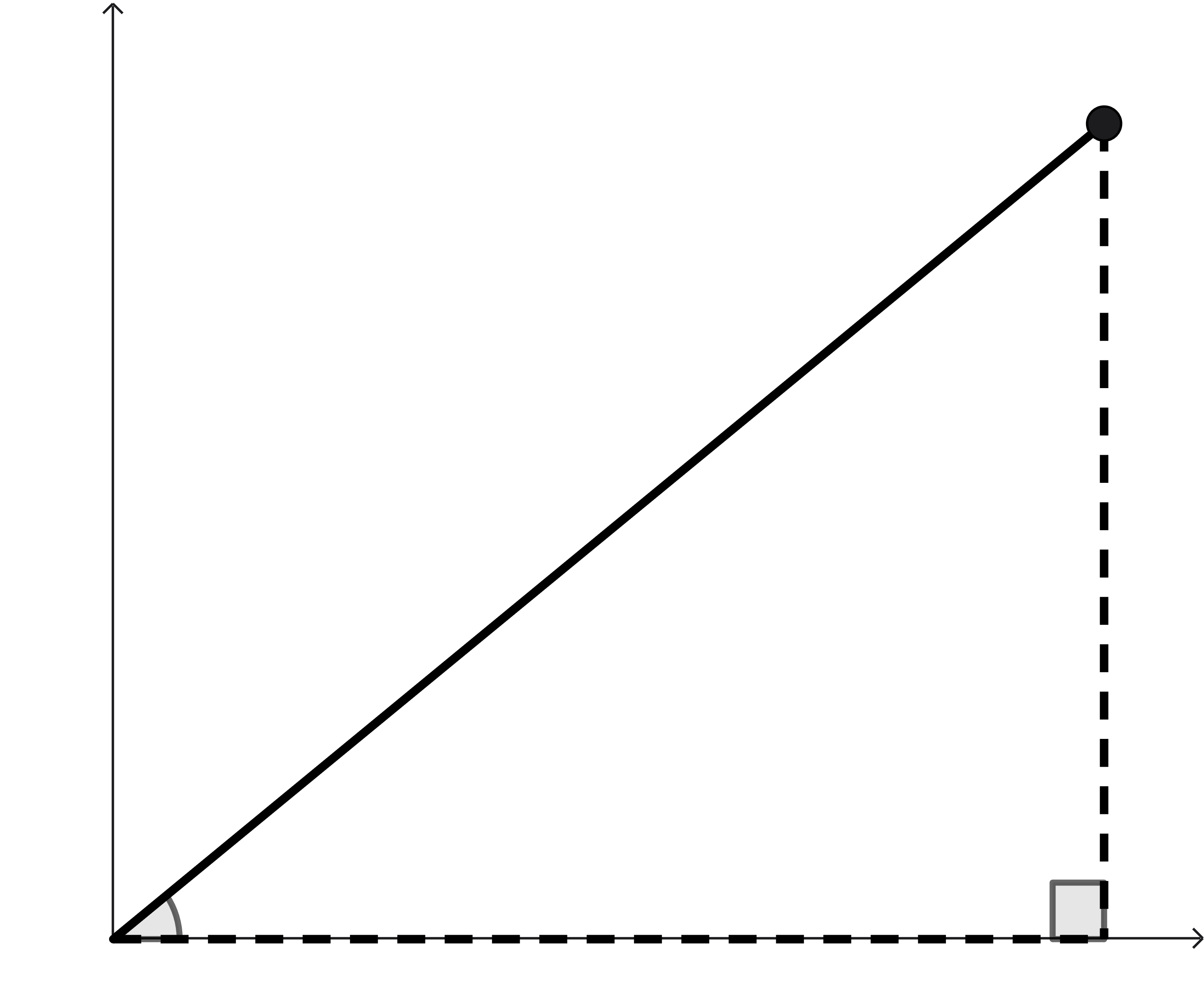
We’re going to think about the two coordinate systems (and converting between them) by considering a point and collecting information. For simplicity, we’ll visualize a point in the first quadrant.
Assume that we know the values of \(x\) and \(y\text{.}\) Come up with an equation linking \(r\text{,}\)\(x\text{,}\) and \(y\) in order for us to find the value of \(r\text{.}\)
Now imagine that we know the values of \(r\) and \(\theta\) instead. Come up with an equation connecting \(x\text{,}\)\(r\text{,}\) and \(\theta\) in order for us to find the value of \(x\text{.}\)
This small triangle exploration gives us a lot of traction! We now have a collection of formulas to help us convert the coordinates of a point back and forth between the Cartesian coordinate system and the polar coordinate system.
We saw in Note 10.2.6 that polar points can be written in an infinite number of ways, and so we need to be careful while solving for \(\theta\) and \(r\) if we are given the Cartesian coordinates \(x\) and \(y\text{.}\)
Note that \(\theta = \tan^{-1}\left(\frac{y}{x}\right)\) will only give values of \(\theta\) in the interval \(\left[-\frac{\pi}{2},\frac{\pi}{2}\right]\text{.}\)
For a Cartesian point in the second or third quadrant, we can either change the value of \(\theta\) to make sure it is pointing in the correct direction, or change the sign on \(r\) to reflect it back into the correct quadrant.
Fill in the following table, converting points written in the Cartesian coordinate system to the polar coordinate system and points in the polar coordinate system to the Cartesian coordinate system. It might be helpful to sketch the point first!
Let’s finish this section with one last note. In thinking about converting the coordinates of a single point, we’ve actually come up with a way of converting functions!
For each of the following polar curves, plot the curve in the graphing utility below. Then, find at least 5 different points on the polar curve, plot them, and describe the behavior of the curve.