
Section 10.1 Parametric Curves

Let’s start with a small deviation from calculus to introduce (or re-introduce) some ideas of how we might define functions and curves. We have been working with functions and graphs of functions for so long, but that might mean that some of the ideas are so engrained that might not even think about them. Let’s remind ourselves as much as possible.

Activity 10.1.1 A Refresher on Functions.

This is mostly a discussion activity. There’s not a lot to do, other than think and share your thoughts with others. If you’re not in a classroom setting, this can be hard! Find someone else with a relatively similar math background, and talk about this with them!

(a)

When you think of a function, what do you think of? What do you imagine in your mind when you hear the word β€œfunction” (in a mathematical context)? Is it based on a definition, a visualization, an example, or some other more loosely connected set of phrases?

(b)

What do you remember about variables? For instance, what is their purpose, their relationship, or their use in defining or visualizing a function?

(c)

How do you visualize a function? What does the picture represent, or how would you explain it to others? What are the important aspects of the visualization that we might use to control what these pictures look like, or what do we try to keep consistent when we visualize these functions? Why do we do this?
None of this should be new to you, but it probably has been some time since you’ve thought about it! The reason we’re starting this chapter (and this section) with this little reminder is simple: we’re going to think about how we could slightly alter some of these basic concepts and change the way that we think about functions, curves, and graphs.

Subsection What If...?

We’re going to try to change some of the assumptions about curves and graphs and functions by asking some β€œWhat if...?” questions. For this section, we’ll ask a very short one:
What if, instead of the \(y\) variable being an output that depends on the \(x\) variable input, we had both \(x\) and \(y\) as outputs of some third variable, like time?
Instead of thinking of \(y\) as a function output of \(x\text{,}\) \(y=f(x)\text{,}\) we’ll think about the vertical component \(y\) and the horizontal component \(x\) of our curve being defined as functions of \(t\text{.}\) Now, instead of \(x\) being an independent variable and \(y\) being dependent on the value of \(x\text{,}\) we have that \(x\) and \(y\) are independent of each other, both dependent on \(t\text{,}\) which we often call a parameter. Typically, we think of this parameter as time: \(x\) and \(y\) both act independently, but change as time marches forward.

Definition 10.1.2 Parametric Curve.

A curve is defined parametrically if
\begin{align*} x \amp = f(t)\\ y \amp = g(t) \end{align*}
for values of \(t\) in some interval.

Aside

This small change in perspective (we’re changing how we view or think of the relationship between variables) impacts a lot of what we assumed and recalled in ActivityΒ 10.1.1.

Subsection Exploring Parametric Curves

Let’s begin with an actual example and see how the parametric definitions can build the curve.

Activity 10.1.3 Our First Parametric Curve.

We’ll begin by exploring the parametrically defined curve:
\begin{align*} x \amp = t^2-3t-4\\ y \amp = 1-t^2 \end{align*}
for \(0 \leq t \leq 4\text{.}\)
For each task, we’ll use the following visualization:

(a)

In Step 1, how does the graph of \(x=t^2-3t-4\) give us information about the horizontal movement of our parametric curve?

(b)

Fill in the table with the \(x\)-values at different values of \(t\text{.}\) Describe the horizontal motion of the parametric curve using this information.

(c)

In Step 2, how does the graph of \(y=1-t^2\) give us information about the vertical movement of our parametric curve?

(d)

Fill in the table with the \(y\)-values at different values of \(t\text{.}\) Describe the vertical motion of the parametric curve using this information.

(e)

In Step 3, confirm that the point follows the path you constructed.
This small interactive graph is a nice one, because it highlights one of the important aspects of a parametric curve: motion. A graph of a parametric curve is really a path that a point travels along, which is pretty different from our original interpretation of a graphβ€”the collection of points \((x,y)\) where \(y=f(x)\text{.}\)

Definition 10.1.4 Orientation.

The direction for which a parametric curve is traced when the value of the parameter is increasing is called the orientation of the curve.
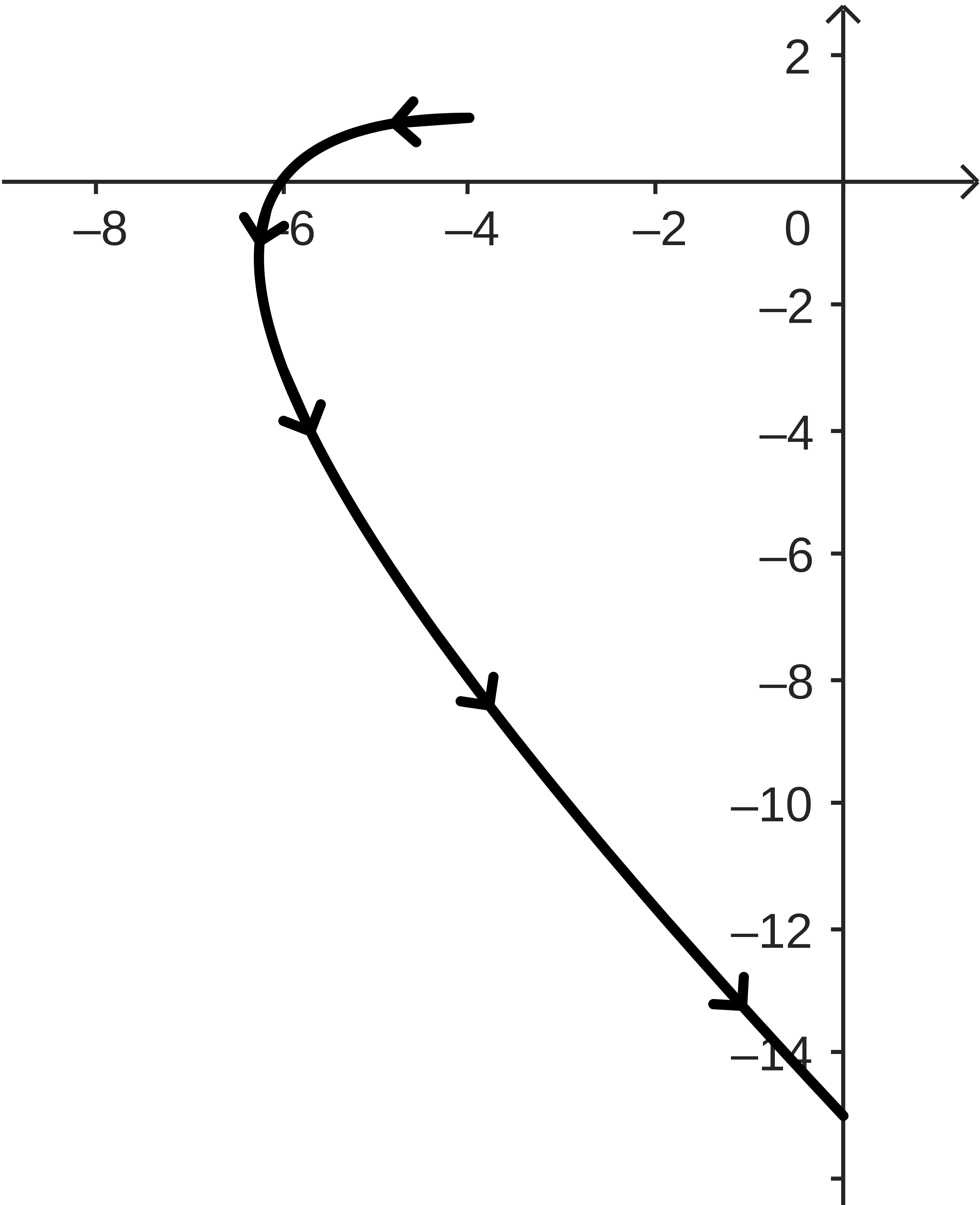
We often try to include some visual clues depicting the orientation or direction of the curve when we visualize it. Often, this can be achieved with a simple animation (where we can see a point move along the curve), but this is also achieved using arrows along a curve.
A parametric curve, shaped a bit like the left side of a  heart. There are arrow heads along the curve, starting on the top and pointing to the left and then downwards as they move along the curve.
Figure 10.1.5. Orientation of a parametric curve: \(\begin{aligned}x \amp = t^2 - 3t-4 \\ y \amp = 1-t^2\end{aligned}\) for \(0 \leq t \leq 4\text{.}\)

Subsection More Parametric Curves

We could end our section with a list of facts or formulas for different curves that we might recognize, but it will be more fun to explore these and discover them ourselves.

Activity 10.1.6 Explore Some Curves.

We’ll start off with a family of parametric curves, where we can change the functions and hopefully predict some of the curve’s behavior.

(a)

Let’s start by thinking about the parametric curve:
\begin{align*} x \amp = \cos(t) \\ y \amp = \sin(t) \end{align*}
for \(0\leq t \leq 2\pi\text{.}\)
Before you visualize any of this, think about the behavior of the \(x\)-values and \(y\)-values. What do you think they’ll do? What will this curve look like?
Visualize the movement of the \(x\)-values, the \(y\)-values, and the complete parametric curve using the graphing tool below.

(b)

What do you think would happen when we multiply the function for \(x\) by a factor of 3?
In the graphing tool above, change the function for \(x\) to:
\begin{equation*} x = 3\cos(t)\text{.} \end{equation*}
Explain the changes you’re seeing.

(c)

What do you think would happen when we multiply the input of the cosine function by 3?
In the graphing tool above, change the function for \(x\) to:
\begin{equation*} x = \cos(3t)\text{.} \end{equation*}
Explain the changes you’re seeing.

(d)

Explore the parametric curve:
\begin{align*} x \amp = \cos(3t)\\ y \amp = \sin(2t) \end{align*}
for \(0 \leq t \leq 2\pi\text{.}\)
Explain to yourself why the curve looks the way that it does.

(e)

Create a parametric curve for a circle, but reverse the orientation.

(f)

Create a parametric curve for a circle centered at the point \((2,-1)\) with radius \(3\text{.}\)

(g)

What do you think the following parametric curve will look like:
\begin{align*} x \amp = \cos^3(t)\\ y \amp = \sin(t) \end{align*}
for \(0 \leq t \leq 2\pi\text{?}\)

Subsection Eliminating the Parameter

It is possible that, in some case, we might want to represent our curve in a more traditional β€œ\(y\) as a function of \(x\)” or β€œ\(x\) as a function of \(y\)” setting. In this case, we need to manipulate our functions for \(x\) and \(y\) in order to eliminate the parameter, \(t\text{,}\) from our function representation.
Typically, this can be done by isolating \(t\) in either the function definition for \(x\) or \(y\text{,}\) and then substituting this new expression for \(t\) into the other variable’s function.

Activity 10.1.7 Eliminate the Parameter.

Consider the parametric curve
\begin{align*} x \amp = \sqrt{t+1}\\ y \amp = \frac{t}{3}+1 \end{align*}
for \(0\leq t \leq 15\text{.}\)

(b)

Substitute this expression for \(t\) into \(y=\dfrac{t}{3}-1\text{.}\)
Solution.
\begin{align*} y \amp = \frac{t}{3}-1\\ \amp = \frac{x^2-1}{3}-1\\ \amp = \frac{x^2}{3}-\frac{4}{3} \end{align*}

(d)

Now substitute this expression for \(t\) into \(x=\sqrt{t+1}\text{.}\)
Solution.
\begin{align*} x \amp = \sqrt{t+1}\\ \amp = \sqrt{(3y+3)+1}\\ \amp = \sqrt{3y+4} \end{align*}

(e)

Use the graphing tool below to check to see if these curves are all the same. You’ll need to find appropriate intervals of \(x\)-values or \(y\)-values along the way.

Activity 10.1.8 Eliminate More Parameters.

For each parametrically-defined curve, eliminate the parameter to create a function \(y=f(x)\) or \(x=f(y)\text{.}\)
Feel free to use the interactive graphing tool in ActivityΒ 10.1.7.

(a)

\(\begin{array}{l} x = t^2-1\\ y = (3t+1)^3 \end{array}\) for \(0 \leq t \leq 2\text{.}\)

(b)

\(\begin{array}{l} x = \ln(t+1)\\ y = \sin(t) \end{array}\) for \(0 \leq t\text{.}\)

(c)

\(\begin{array}{l} x = \cos^2(t)\\ y = (t+1)^{3/2} \end{array}\) for \(0 \leq t\text{.}\)

(d)

\(\begin{array}{l} x = \tan^{-1}(x)\\ y = t^2 \end{array}\) for \(-2 \leq t \leq 2\text{.}\)
We might notice that this strategy depends on us being able to solve for \(t\) in at least one of these functions. For instance, the following parametric curve will be hard to employ this strategy:
\begin{align*} x \amp = t - \sin(t)\\ y \amp = t\cos(t) \end{align*}
There are no β€œnice” ways of solving for \(t\) in either of these functions!
This is everything we need for now. We’re going to make one more quick stop to check out another way of representing functions, and then we’ll spend our time thinking about how we might do calculus with these parametric curves.

Practice Problems Practice Problems

1.

Explain how a curve written in parametric form is different than one written in standard function notation.

2.

For each of the following parametric curves, plot the curves in the graphing utility below. Then, find at least 5 different points on the curve, plot them, and describe the curve.

(a)

\(\begin{array}{l} x=t-4\\ y=3+t-t^2 \end{array}\) for \(0\leq t\leq 10\text{.}\)

(b)

\(\begin{array}{l} x = t+3\\ y = 5-2t \end{array}\) for \(0\leq t\leq 5\text{.}\)

(c)

\(\begin{array}{l} x=5\cos^2(t)\\ y=5\sin^2(t) \end{array}\) for \(0\leq t\leq 2\pi\text{.}\)

(d)

\(\begin{array}{l} x=\sqrt{t+4}\\ y=5t+1 \end{array}\) for \(0\leq t\leq 5\text{.}\)

3.

Eliminate the parameter, \(t\text{,}\) in each of the parametric curves, expressing the curve either as a function \(y=f(x)\) or \(x=f(y)\text{.}\)

(a)

\(\begin{array}{l} x=t-4\\ y=3+t-t^2 \end{array}\) for \(0\leq t\leq 10\text{.}\)

(b)

\(\begin{array}{l} x = t+3\\ y = 5-2t \end{array}\) for \(0\leq t\leq 5\text{.}\)

(c)

\(\begin{array}{l} x=5\cos^2(t)\\ y=5\sin^2(t) \end{array}\) for \(0\leq t\leq 2\pi\text{.}\)

(d)

\(\begin{array}{l} x=\sqrt{t+4}\\ y=5t+1 \end{array}\) for \(0\leq t\leq 5\text{.}\)

4.

In ActivityΒ 10.1.6Β Explore Some Curves, we saw the we can define a circle parametrically by
\begin{align*} x \amp = \cos(t)\\ y \amp = \sin(t) \end{align*}
for \(0\leq t \leq 2\pi\text{.}\)

(a)

Remind yourself why this parametric definition makes sense, based on how we think about trig functions on a unit circle.

(b)

Eliminate the parameter to create an equation with \(x\) and \(y\) related to each other.
Hint.
Try squaring each parametric function! How can you combine them in a typical trigonometric identity way?

(c)

How does the function \(f(t)=\cos(5t)\) compare to the function \(g(t)=\cos(t)\text{?}\) How about \(\ell(t)=\sin(5t)\) compared to the function \(m(t)=\sin(t)\text{?}\)
(d)

The parametric curve
\begin{align*} x \amp = \cos(5t)\\ y \amp = \sin(5t) \end{align*}
for \(0 \leq t \leq 2\pi\) looks exactly the same as the unit circle we defined earlier.
How is it different? What does the coefficient on \(t\) do?

(e)

Create a parametric curve that looks like the unit circle but has an opposite orientation (direction).

